Analysis
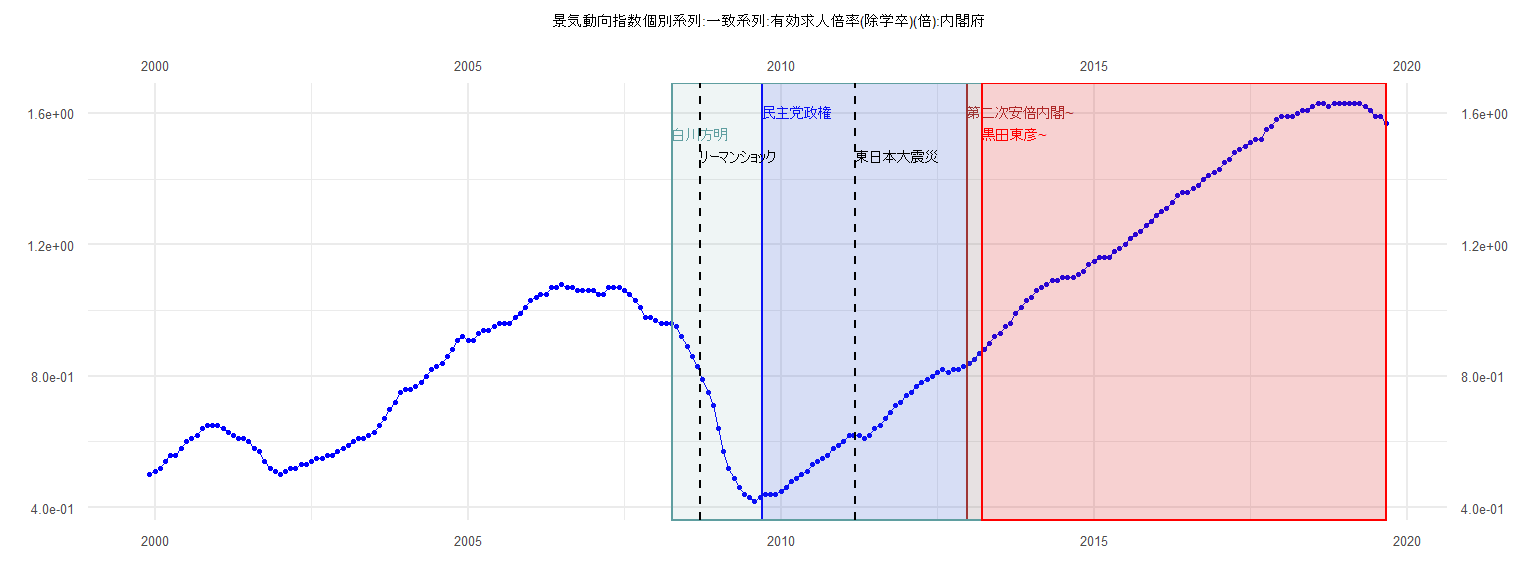
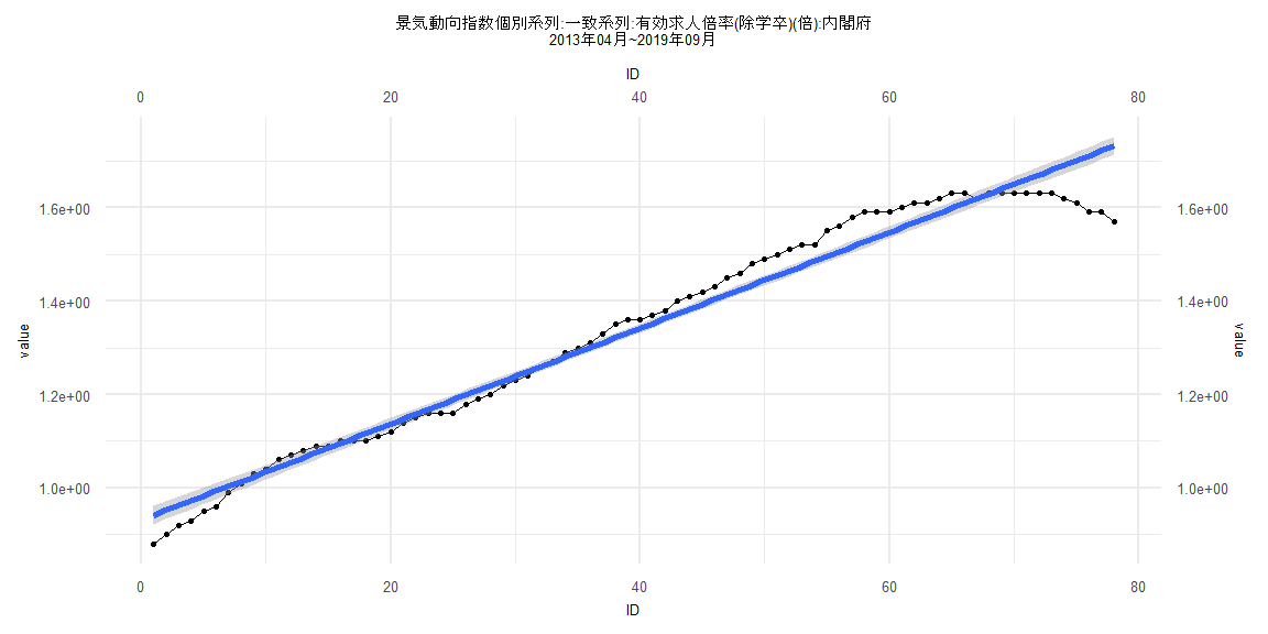
[1] "景気動向指数個別系列:一致系列:有効求人倍率(除学卒)(倍):内閣府"
      Jan  Feb  Mar  Apr  May  Jun  Jul  Aug  Sep  Oct  Nov  Dec
1999                                                        0.50
2000 0.51 0.52 0.54 0.56 0.56 0.58 0.60 0.61 0.62 0.64 0.65 0.65
2001 0.65 0.64 0.63 0.62 0.61 0.61 0.60 0.58 0.57 0.54 0.52 0.51
2002 0.50 0.51 0.52 0.52 0.53 0.53 0.54 0.55 0.55 0.56 0.56 0.57
2003 0.58 0.59 0.60 0.61 0.61 0.62 0.63 0.65 0.67 0.70 0.72 0.75
2004 0.76 0.76 0.77 0.78 0.80 0.82 0.83 0.84 0.86 0.88 0.91 0.92
2005 0.91 0.91 0.93 0.94 0.94 0.95 0.96 0.96 0.96 0.98 0.99 1.01
2006 1.03 1.04 1.05 1.05 1.07 1.07 1.08 1.07 1.07 1.06 1.06 1.06
2007 1.06 1.05 1.05 1.07 1.07 1.07 1.06 1.05 1.03 1.01 0.98 0.98
2008 0.97 0.96 0.96 0.96 0.95 0.92 0.89 0.86 0.83 0.79 0.75 0.71
2009 0.64 0.57 0.52 0.49 0.46 0.44 0.43 0.42 0.43 0.44 0.44 0.44
2010 0.45 0.46 0.48 0.49 0.50 0.51 0.53 0.54 0.55 0.56 0.58 0.59
2011 0.60 0.62 0.62 0.62 0.61 0.62 0.64 0.65 0.67 0.69 0.71 0.72
2012 0.74 0.75 0.77 0.78 0.79 0.80 0.81 0.82 0.81 0.82 0.82 0.83
2013 0.84 0.85 0.87 0.88 0.90 0.92 0.93 0.95 0.96 0.99 1.01 1.03
2014 1.04 1.06 1.07 1.08 1.09 1.09 1.10 1.10 1.10 1.11 1.12 1.14
2015 1.15 1.16 1.16 1.16 1.18 1.19 1.20 1.22 1.23 1.24 1.26 1.27
2016 1.29 1.30 1.31 1.33 1.35 1.36 1.36 1.37 1.38 1.40 1.41 1.42
2017 1.43 1.45 1.46 1.48 1.49 1.50 1.51 1.52 1.52 1.55 1.56 1.58
2018 1.59 1.59 1.59 1.60 1.61 1.61 1.62 1.63 1.63 1.62 1.63 1.63
2019 1.63 1.63 1.63 1.63 1.62 1.61 1.59 1.59 1.57
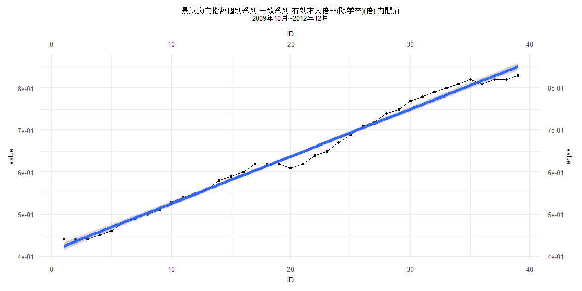
Call:
lm(formula = value ~ ID)

Residuals:
      Min        1Q    Median        3Q       Max
-0.028945 -0.007692  0.002332  0.010428  0.019777

Coefficients:
            Estimate Std. Error t value            Pr(>|t|)
(Intercept) 0.412632   0.004406   93.66 <0.0000000000000002 ***
ID          0.011253   0.000192   58.62 <0.0000000000000002 ***
---
Signif. codes:  0 '***' 0.001 '**' 0.01 '*' 0.05 '.' 0.1 ' ' 1

Residual standard error: 0.01349 on 37 degrees of freedom
Multiple R-squared:  0.9893,    Adjusted R-squared:  0.9891
F-statistic:  3436 on 1 and 37 DF,  p-value: < 0.00000000000000022


    Two-sample Kolmogorov-Smirnov test

data:  lm_residuals and rnorm(n = length(lm_residuals), mean = 0, sd = sd(lm_residuals))
D = 0.12821, p-value = 0.9114
alternative hypothesis: two-sided


    Durbin-Watson test

data:  value ~ ID
DW = 0.34659, p-value = 0.00000000000133
alternative hypothesis: true autocorrelation is greater than 0


    studentized Breusch-Pagan test

data:  value ~ ID
BP = 5.6803, df = 1, p-value = 0.01716


    Box-Ljung test

data:  lm_residuals
X-squared = 25.151, df = 1, p-value = 0.0000005301
Call:
lm(formula = value ~ ID)

Residuals:
     Min       1Q   Median       3Q      Max
-0.16634 -0.01409  0.01071  0.02933  0.06282

Coefficients:
             Estimate Std. Error t value            Pr(>|t|)
(Intercept) 0.8910000  0.0098311   90.63 <0.0000000000000002 ***
ID          0.0104363  0.0002083   50.10 <0.0000000000000002 ***
---
Signif. codes:  0 '***' 0.001 '**' 0.01 '*' 0.05 '.' 0.1 ' ' 1

Residual standard error: 0.04383 on 79 degrees of freedom
Multiple R-squared:  0.9695,    Adjusted R-squared:  0.9691
F-statistic:  2510 on 1 and 79 DF,  p-value: < 0.00000000000000022


    Two-sample Kolmogorov-Smirnov test

data:  lm_residuals and rnorm(n = length(lm_residuals), mean = 0, sd = sd(lm_residuals))
D = 0.1358, p-value = 0.4462
alternative hypothesis: two-sided


    Durbin-Watson test

data:  value ~ ID
DW = 0.048602, p-value < 0.00000000000000022
alternative hypothesis: true autocorrelation is greater than 0


    studentized Breusch-Pagan test

data:  value ~ ID
BP = 13.131, df = 1, p-value = 0.0002905


    Box-Ljung test

data:  lm_residuals
X-squared = 63.917, df = 1, p-value = 0.000000000000001332
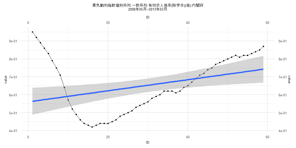
Call:
lm(formula = value ~ ID)

Residuals:
     Min       1Q   Median       3Q      Max
-0.18986 -0.11065 -0.03390  0.09099  0.38642

Coefficients:
            Estimate Std. Error t value             Pr(>|t|)
(Intercept) 0.560491   0.038398  14.597 < 0.0000000000000002 ***
ID          0.003085   0.001113   2.772              0.00752 **
---
Signif. codes:  0 '***' 0.001 '**' 0.01 '*' 0.05 '.' 0.1 ' ' 1

Residual standard error: 0.1456 on 57 degrees of freedom
Multiple R-squared:  0.1188,    Adjusted R-squared:  0.1033
F-statistic: 7.683 on 1 and 57 DF,  p-value: 0.007517


    Two-sample Kolmogorov-Smirnov test

data:  lm_residuals and rnorm(n = length(lm_residuals), mean = 0, sd = sd(lm_residuals))
D = 0.13559, p-value = 0.6544
alternative hypothesis: two-sided


    Durbin-Watson test

data:  value ~ ID
DW = 0.025858, p-value < 0.00000000000000022
alternative hypothesis: true autocorrelation is greater than 0


    studentized Breusch-Pagan test

data:  value ~ ID
BP = 22.327, df = 1, p-value = 0.0000023


    Box-Ljung test

data:  lm_residuals
X-squared = 52.356, df = 1, p-value = 0.0000000000004629
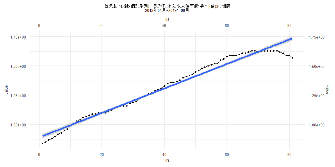
Call:
lm(formula = value ~ ID)

Residuals:
      Min        1Q    Median        3Q       Max
-0.161659 -0.017568  0.005123  0.028525  0.063722

Coefficients:
             Estimate Std. Error t value            Pr(>|t|)
(Intercept) 0.9316750  0.0098050   95.02 <0.0000000000000002 ***
ID          0.0102562  0.0002157   47.56 <0.0000000000000002 ***
---
Signif. codes:  0 '***' 0.001 '**' 0.01 '*' 0.05 '.' 0.1 ' ' 1

Residual standard error: 0.04288 on 76 degrees of freedom
Multiple R-squared:  0.9675,    Adjusted R-squared:  0.9671
F-statistic:  2262 on 1 and 76 DF,  p-value: < 0.00000000000000022


    Two-sample Kolmogorov-Smirnov test

data:  lm_residuals and rnorm(n = length(lm_residuals), mean = 0, sd = sd(lm_residuals))
D = 0.17949, p-value = 0.1624
alternative hypothesis: two-sided


    Durbin-Watson test

data:  value ~ ID
DW = 0.051849, p-value < 0.00000000000000022
alternative hypothesis: true autocorrelation is greater than 0


    studentized Breusch-Pagan test

data:  value ~ ID
BP = 14.617, df = 1, p-value = 0.0001317


    Box-Ljung test

data:  lm_residuals
X-squared = 60.896, df = 1, p-value = 0.000000000000005995