Analysis
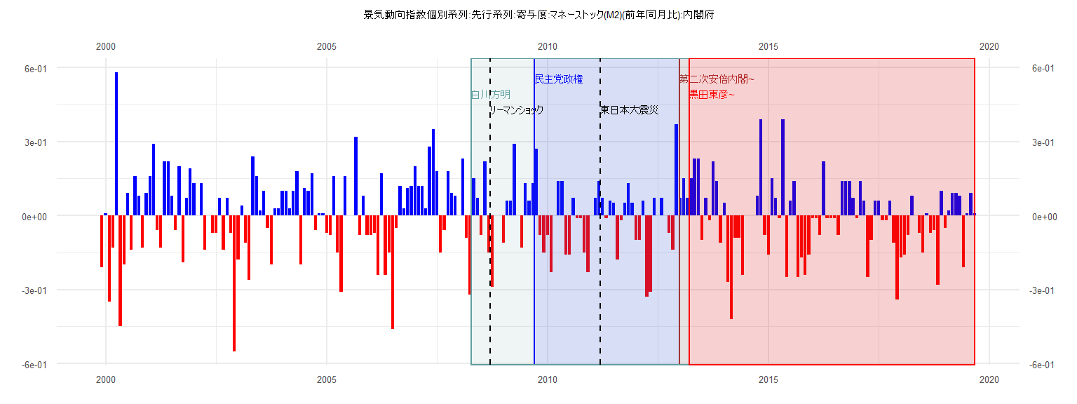
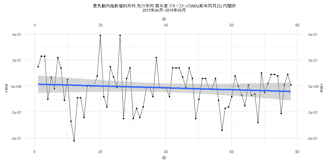
[1] "景気動向指数個別系列:先行系列:寄与度:マネーストック(M2)(前年同月比):内閣府"
       Jan   Feb   Mar   Apr   May   Jun   Jul   Aug   Sep   Oct   Nov   Dec
1999                                                                   -0.21
2000  0.01 -0.35 -0.13  0.58 -0.45 -0.20  0.09 -0.14  0.16  0.08 -0.13  0.09
2001  0.16  0.29 -0.06 -0.13  0.22  0.22  0.08 -0.06  0.20 -0.19  0.07  0.19
2002  0.13  0.00  0.13 -0.14  0.00 -0.07 -0.07  0.07 -0.14  0.07 -0.07 -0.55
2003 -0.18  0.04 -0.11 -0.26  0.24  0.16  0.02  0.10 -0.05 -0.20  0.03  0.03
2004  0.10  0.10  0.03  0.10  0.18 -0.20  0.11  0.10  0.17 -0.06  0.01  0.01
2005 -0.07 -0.08  0.16 -0.15 -0.31  0.16  0.00  0.00  0.32 -0.08  0.08 -0.08
2006 -0.08 -0.07 -0.24  0.17 -0.24 -0.15 -0.46 -0.05  0.12  0.03  0.11  0.12
2007  0.20  0.12  0.12  0.03  0.28  0.35  0.18 -0.15 -0.06  0.18  0.09  0.08
2008  0.00  0.23 -0.09 -0.32  0.15  0.07 -0.08  0.22 -0.15 -0.29  0.00  0.00
2009 -0.11  0.06  0.06  0.29  0.00 -0.13  0.13  0.06  0.13  0.27 -0.08 -0.15
2010 -0.08 -0.23  0.00  0.14  0.14 -0.16 -0.16  0.07 -0.01 -0.01 -0.15 -0.23
2011  0.00  0.07  0.14  0.07 -0.01  0.06  0.05 -0.18 -0.02  0.05  0.13  0.05
2012 -0.10 -0.10  0.06 -0.33 -0.31  0.07  0.00  0.07  0.00 -0.07 -0.14  0.37
2013  0.07  0.15  0.07  0.15  0.23  0.23 -0.10  0.07 -0.02  0.22  0.14 -0.11
2014  0.05 -0.27 -0.42 -0.09 -0.09 -0.24  0.00  0.00  0.00  0.08  0.39 -0.08
2015 -0.16  0.15  0.07 -0.01  0.39 -0.25  0.06  0.14 -0.25 -0.17 -0.24 -0.16
2016 -0.01 -0.01 -0.08  0.22 -0.01 -0.01 -0.01 -0.08  0.14  0.14  0.14  0.07
2017 -0.01  0.14  0.06 -0.25 -0.10  0.06  0.06 -0.02 -0.02  0.06 -0.11 -0.34
2018 -0.17 -0.16 -0.08  0.08  0.00 -0.07 -0.15  0.01 -0.07 -0.06 -0.28  0.10
2019 -0.05  0.02  0.09  0.09  0.08 -0.21  0.01  0.09  0.01
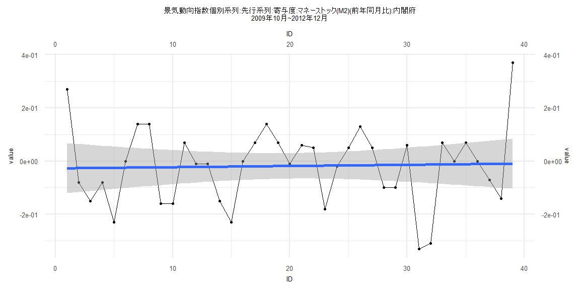
Call:
lm(formula = value ~ ID)

Residuals:
     Min       1Q   Median       3Q      Max
-0.31672 -0.10501  0.01178  0.08194  0.37971

Coefficients:
              Estimate Std. Error t value Pr(>|t|)
(Intercept) -0.0271525  0.0482569  -0.563    0.577
ID           0.0004474  0.0021028   0.213    0.833

Residual standard error: 0.1478 on 37 degrees of freedom
Multiple R-squared:  0.001222,  Adjusted R-squared:  -0.02577
F-statistic: 0.04526 on 1 and 37 DF,  p-value: 0.8327


    Two-sample Kolmogorov-Smirnov test

data:  lm_residuals and rnorm(n = length(lm_residuals), mean = 0, sd = sd(lm_residuals))
D = 0.17949, p-value = 0.5622
alternative hypothesis: two-sided


    Durbin-Watson test

data:  value ~ ID
DW = 1.4939, p-value = 0.03625
alternative hypothesis: true autocorrelation is greater than 0


    studentized Breusch-Pagan test

data:  value ~ ID
BP = 0.58251, df = 1, p-value = 0.4453


    Box-Ljung test

data:  lm_residuals
X-squared = 0.50369, df = 1, p-value = 0.4779
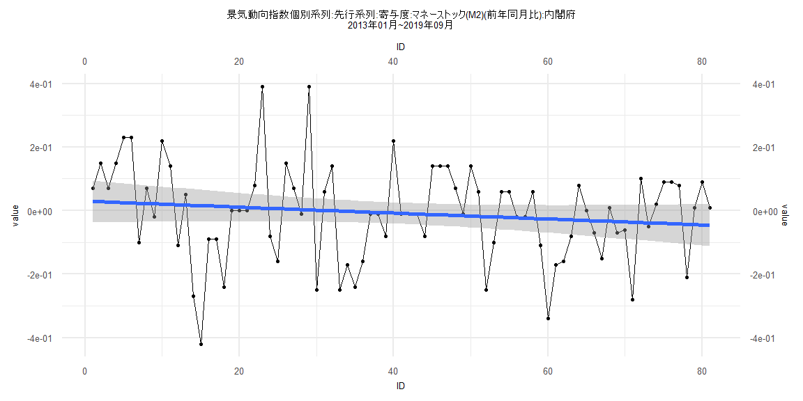
Call:
lm(formula = value ~ ID)

Residuals:
     Min       1Q   Median       3Q      Max
-0.43572 -0.08733  0.00250  0.10996  0.38733

Coefficients:
              Estimate Std. Error t value Pr(>|t|)
(Intercept)  0.0297037  0.0338354   0.878    0.383
ID          -0.0009322  0.0007169  -1.300    0.197

Residual standard error: 0.1509 on 79 degrees of freedom
Multiple R-squared:  0.02096,   Adjusted R-squared:  0.008565
F-statistic: 1.691 on 1 and 79 DF,  p-value: 0.1972


    Two-sample Kolmogorov-Smirnov test

data:  lm_residuals and rnorm(n = length(lm_residuals), mean = 0, sd = sd(lm_residuals))
D = 0.12346, p-value = 0.5705
alternative hypothesis: two-sided


    Durbin-Watson test

data:  value ~ ID
DW = 1.6142, p-value = 0.03041
alternative hypothesis: true autocorrelation is greater than 0


    studentized Breusch-Pagan test

data:  value ~ ID
BP = 2.9248, df = 1, p-value = 0.08723


    Box-Ljung test

data:  lm_residuals
X-squared = 3.0834, df = 1, p-value = 0.0791
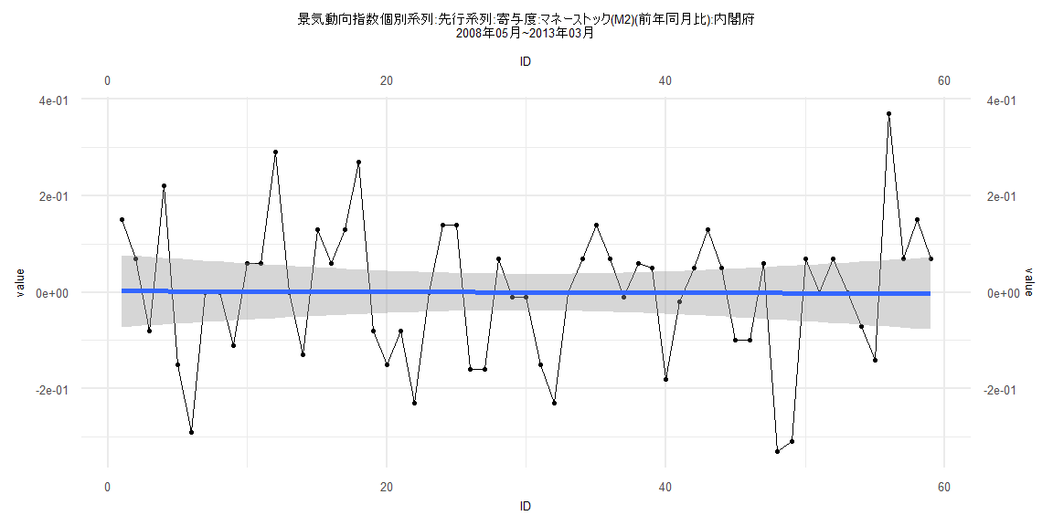
Call:
lm(formula = value ~ ID)

Residuals:
     Min       1Q   Median       3Q      Max
-0.32831 -0.09852  0.00195  0.07195  0.37237

Coefficients:
               Estimate  Std. Error t value Pr(>|t|)
(Intercept)  0.00237288  0.03827736   0.062    0.951
ID          -0.00008475  0.00110961  -0.076    0.939

Residual standard error: 0.1451 on 57 degrees of freedom
Multiple R-squared:  0.0001023, Adjusted R-squared:  -0.01744
F-statistic: 0.005833 on 1 and 57 DF,  p-value: 0.9394


    Two-sample Kolmogorov-Smirnov test

data:  lm_residuals and rnorm(n = length(lm_residuals), mean = 0, sd = sd(lm_residuals))
D = 0.15254, p-value = 0.5021
alternative hypothesis: two-sided


    Durbin-Watson test

data:  value ~ ID
DW = 1.6336, p-value = 0.05886
alternative hypothesis: true autocorrelation is greater than 0


    studentized Breusch-Pagan test

data:  value ~ ID
BP = 0.051074, df = 1, p-value = 0.8212


    Box-Ljung test

data:  lm_residuals
X-squared = 1.834, df = 1, p-value = 0.1757
Call:
lm(formula = value ~ ID)

Residuals:
     Min       1Q   Median       3Q      Max
-0.42726 -0.09325  0.00225  0.10268  0.39283

Coefficients:
              Estimate Std. Error t value Pr(>|t|)
(Intercept)  0.0159074  0.0349625   0.455    0.650
ID          -0.0007208  0.0007690  -0.937    0.352

Residual standard error: 0.1529 on 76 degrees of freedom
Multiple R-squared:  0.01143,   Adjusted R-squared:  -0.001579
F-statistic: 0.8786 on 1 and 76 DF,  p-value: 0.3516


    Two-sample Kolmogorov-Smirnov test

data:  lm_residuals and rnorm(n = length(lm_residuals), mean = 0, sd = sd(lm_residuals))
D = 0.15385, p-value = 0.316
alternative hypothesis: two-sided


    Durbin-Watson test

data:  value ~ ID
DW = 1.6222, p-value = 0.03531
alternative hypothesis: true autocorrelation is greater than 0


    studentized Breusch-Pagan test

data:  value ~ ID
BP = 4.3851, df = 1, p-value = 0.03625


    Box-Ljung test

data:  lm_residuals
X-squared = 2.7154, df = 1, p-value = 0.09938