Analysis
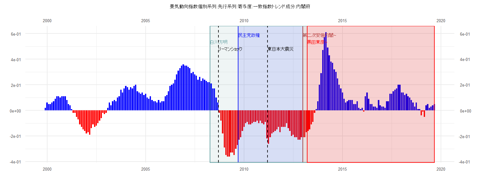
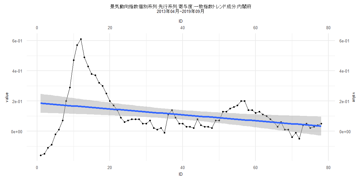
[1] "景気動向指数個別系列:先行系列:寄与度:一致指数トレンド成分:内閣府"
       Jan   Feb   Mar   Apr   May   Jun   Jul   Aug   Sep   Oct   Nov   Dec
1999                                                                    0.02
2000  0.06  0.05  0.05  0.06  0.07  0.09  0.11  0.11  0.10  0.11  0.11  0.11
2001  0.08  0.05  0.04  0.01 -0.02 -0.02 -0.05 -0.07 -0.11 -0.13 -0.15 -0.16
2002 -0.18 -0.17 -0.19 -0.14 -0.11 -0.13 -0.12 -0.10 -0.08 -0.06 -0.02 -0.03
2003 -0.02  0.02  0.06  0.04  0.07  0.08  0.07  0.10  0.11  0.16  0.14  0.17
2004  0.19  0.18  0.16  0.18  0.17  0.19  0.20  0.15  0.14  0.13  0.14  0.12
2005  0.13  0.10  0.09  0.11  0.08  0.07  0.07  0.06  0.08  0.06  0.07  0.07
2006  0.11  0.12  0.15  0.19  0.20  0.21  0.24  0.28  0.31  0.33  0.35  0.36
2007  0.35  0.35  0.34  0.33  0.29  0.30  0.28  0.27  0.24  0.26  0.23  0.25
2008  0.24  0.23  0.22  0.22  0.21  0.17  0.17  0.10  0.06 -0.02 -0.08 -0.18
2009 -0.29 -0.35 -0.36 -0.36 -0.33 -0.33 -0.35 -0.30 -0.27 -0.23 -0.21 -0.16
2010 -0.13 -0.10 -0.09 -0.11 -0.11 -0.10 -0.09 -0.09 -0.08 -0.10 -0.08 -0.10
2011 -0.11 -0.09 -0.22 -0.26 -0.21 -0.18 -0.17 -0.16 -0.15 -0.13 -0.17 -0.13
2012 -0.13 -0.13 -0.10 -0.14 -0.16 -0.20 -0.19 -0.21 -0.21 -0.23 -0.23 -0.21
2013 -0.21 -0.21 -0.17 -0.16 -0.15 -0.11 -0.09 -0.02  0.01  0.07  0.20  0.29
2014  0.47  0.57  0.61  0.49  0.43  0.38  0.37  0.32  0.30  0.25  0.20  0.17
2015  0.14  0.09  0.06  0.07  0.08  0.08  0.08  0.05  0.05  0.07  0.02  0.01
2016  0.02 -0.01  0.11  0.14  0.09  0.05  0.05  0.03  0.03  0.02  0.08  0.04
2017  0.03  0.03  0.02  0.07  0.07  0.13  0.13  0.15  0.16  0.17  0.20  0.20
2018  0.14  0.14  0.12  0.13  0.11  0.10  0.08  0.06  0.03  0.06  0.01  0.01
2019 -0.04 -0.01 -0.05  0.04  0.05  0.02  0.03  0.04  0.05
Call:
lm(formula = value ~ ID)

Residuals:
     Min       1Q   Median       3Q      Max
-0.11587 -0.02710  0.01475  0.03595  0.07084

Coefficients:
              Estimate Std. Error t value     Pr(>|t|)
(Intercept) -0.1121727  0.0156450  -7.170 0.0000000169 ***
ID          -0.0019555  0.0006817  -2.868      0.00678 **
---
Signif. codes:  0 '***' 0.001 '**' 0.01 '*' 0.05 '.' 0.1 ' ' 1

Residual standard error: 0.04791 on 37 degrees of freedom
Multiple R-squared:  0.1819,    Adjusted R-squared:  0.1598
F-statistic: 8.228 on 1 and 37 DF,  p-value: 0.006776


    Two-sample Kolmogorov-Smirnov test

data:  lm_residuals and rnorm(n = length(lm_residuals), mean = 0, sd = sd(lm_residuals))
D = 0.15385, p-value = 0.7523
alternative hypothesis: two-sided


    Durbin-Watson test

data:  value ~ ID
DW = 0.45939, p-value = 0.0000000002934
alternative hypothesis: true autocorrelation is greater than 0


    studentized Breusch-Pagan test

data:  value ~ ID
BP = 3.6351, df = 1, p-value = 0.05657


    Box-Ljung test

data:  lm_residuals
X-squared = 19.949, df = 1, p-value = 0.000007953
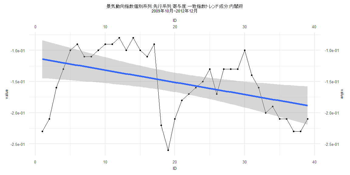
Call:
lm(formula = value ~ ID)

Residuals:
     Min       1Q   Median       3Q      Max
-0.34578 -0.06047 -0.02218  0.05593  0.48743

Coefficients:
              Estimate Std. Error t value Pr(>|t|)
(Intercept)  0.1367284  0.0346948   3.941 0.000174 ***
ID          -0.0009440  0.0007351  -1.284 0.202829
---
Signif. codes:  0 '***' 0.001 '**' 0.01 '*' 0.05 '.' 0.1 ' ' 1

Residual standard error: 0.1547 on 79 degrees of freedom
Multiple R-squared:  0.02045,   Adjusted R-squared:  0.008049
F-statistic: 1.649 on 1 and 79 DF,  p-value: 0.2028


    Two-sample Kolmogorov-Smirnov test

data:  lm_residuals and rnorm(n = length(lm_residuals), mean = 0, sd = sd(lm_residuals))
D = 0.1358, p-value = 0.4462
alternative hypothesis: two-sided


    Durbin-Watson test

data:  value ~ ID
DW = 0.094466, p-value < 0.00000000000000022
alternative hypothesis: true autocorrelation is greater than 0


    studentized Breusch-Pagan test

data:  value ~ ID
BP = 25.508, df = 1, p-value = 0.0000004406


    Box-Ljung test

data:  lm_residuals
X-squared = 71.301, df = 1, p-value < 0.00000000000000022
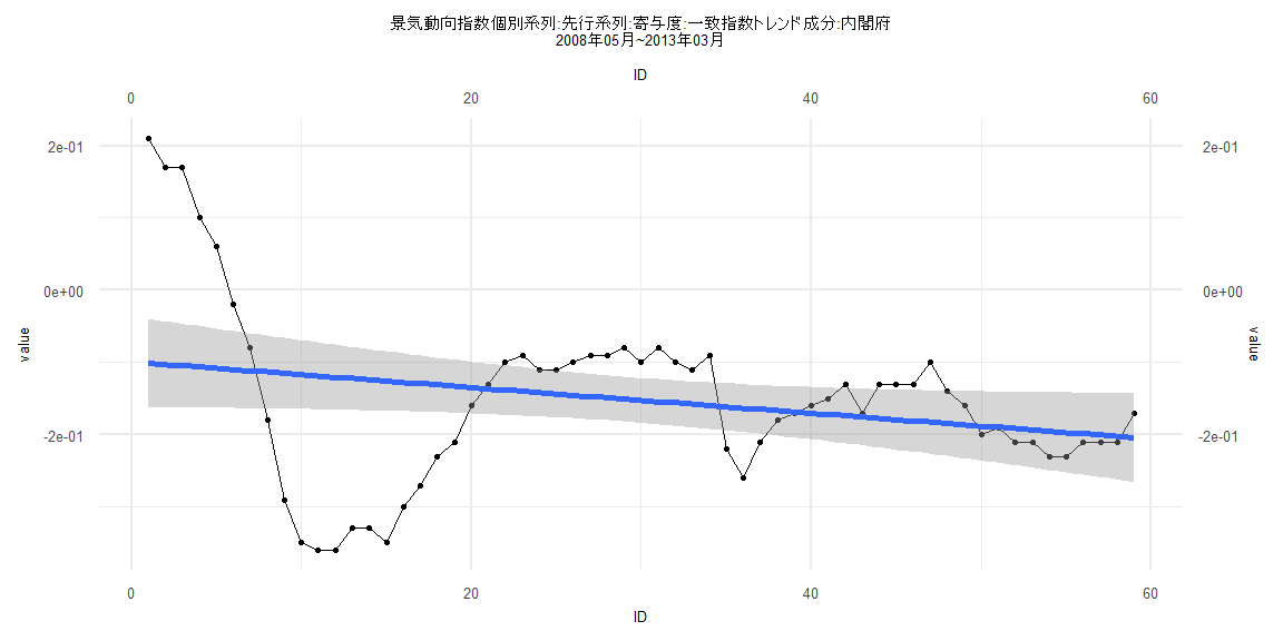
Call:
lm(formula = value ~ ID)

Residuals:
     Min       1Q   Median       3Q      Max
-0.24126 -0.03988  0.01033  0.05055  0.31095

Coefficients:
              Estimate Std. Error t value Pr(>|t|)
(Intercept) -0.0991701  0.0314411  -3.154  0.00257 **
ID          -0.0017791  0.0009114  -1.952  0.05586 .
---
Signif. codes:  0 '***' 0.001 '**' 0.01 '*' 0.05 '.' 0.1 ' ' 1

Residual standard error: 0.1192 on 57 degrees of freedom
Multiple R-squared:  0.06266,   Adjusted R-squared:  0.04621
F-statistic:  3.81 on 1 and 57 DF,  p-value: 0.05586


    Two-sample Kolmogorov-Smirnov test

data:  lm_residuals and rnorm(n = length(lm_residuals), mean = 0, sd = sd(lm_residuals))
D = 0.23729, p-value = 0.07193
alternative hypothesis: two-sided


    Durbin-Watson test

data:  value ~ ID
DW = 0.11039, p-value < 0.00000000000000022
alternative hypothesis: true autocorrelation is greater than 0


    studentized Breusch-Pagan test

data:  value ~ ID
BP = 26.961, df = 1, p-value = 0.0000002077


    Box-Ljung test

data:  lm_residuals
X-squared = 48.536, df = 1, p-value = 0.000000000003243
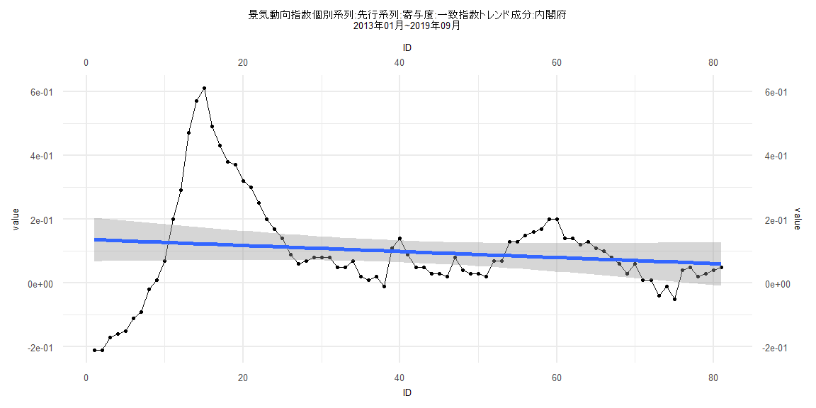
Call:
lm(formula = value ~ ID)

Residuals:
     Min       1Q   Median       3Q      Max
-0.34496 -0.07146 -0.01919  0.05199  0.44664

Coefficients:
              Estimate Std. Error t value    Pr(>|t|)
(Intercept)  0.1869264  0.0321825   5.808 0.000000139 ***
ID          -0.0019637  0.0007078  -2.774     0.00696 **
---
Signif. codes:  0 '***' 0.001 '**' 0.01 '*' 0.05 '.' 0.1 ' ' 1

Residual standard error: 0.1407 on 76 degrees of freedom
Multiple R-squared:  0.09196,   Adjusted R-squared:  0.08001
F-statistic: 7.697 on 1 and 76 DF,  p-value: 0.006958


    Two-sample Kolmogorov-Smirnov test

data:  lm_residuals and rnorm(n = length(lm_residuals), mean = 0, sd = sd(lm_residuals))
D = 0.17949, p-value = 0.1624
alternative hypothesis: two-sided


    Durbin-Watson test

data:  value ~ ID
DW = 0.11784, p-value < 0.00000000000000022
alternative hypothesis: true autocorrelation is greater than 0


    studentized Breusch-Pagan test

data:  value ~ ID
BP = 24.396, df = 1, p-value = 0.0000007844


    Box-Ljung test

data:  lm_residuals
X-squared = 65.857, df = 1, p-value = 0.0000000000000004441