Analysis
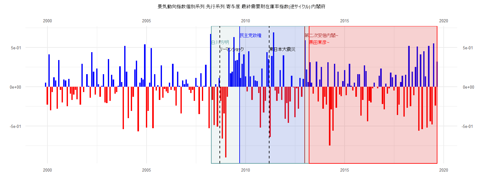
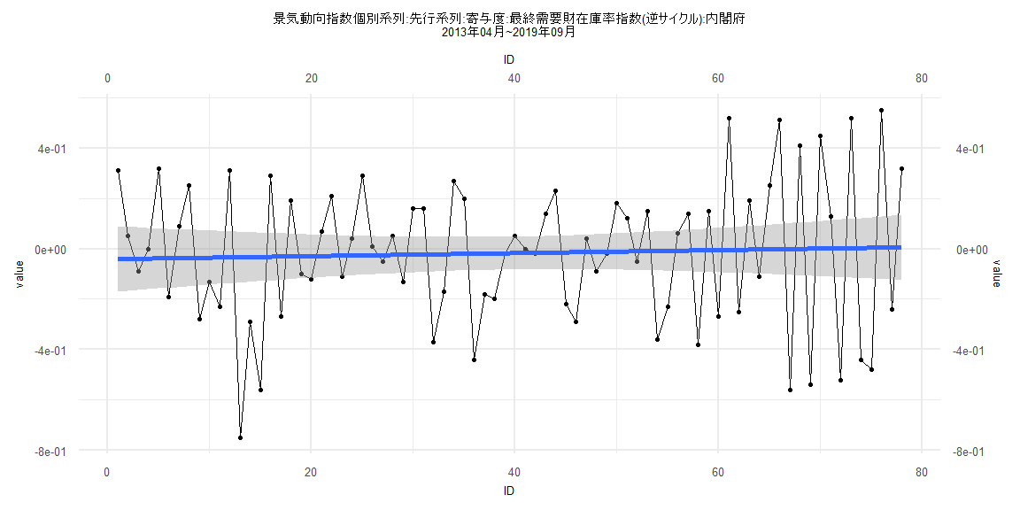
[1] "景気動向指数個別系列:先行系列:寄与度:最終需要財在庫率指数(逆サイクル):内閣府"
       Jan   Feb   Mar   Apr   May   Jun   Jul   Aug   Sep   Oct   Nov   Dec
1999                                                                    0.05
2000 -0.23  0.41 -0.30 -0.07  0.12  0.08 -0.28  0.34 -0.04 -0.20  0.09  0.08
2001 -0.25  0.10 -0.09 -0.17 -0.10 -0.04 -0.16  0.00 -0.23  0.29 -0.07  0.00
2002  0.16  0.01 -0.14  0.44  0.19 -0.10  0.23  0.03 -0.13  0.01  0.16 -0.20
2003 -0.21  0.35 -0.18  0.15  0.09 -0.09 -0.07  0.01  0.26  0.06 -0.54  0.52
2004  0.19 -0.40  0.00 -0.31 -0.13  0.22  0.33 -0.57  0.05  0.11  0.09  0.54
2005 -0.52 -0.31  0.05  0.49 -0.53  0.16 -0.05  0.02 -0.17  0.27 -0.14 -0.03
2006 -0.06 -0.08  0.05 -0.04  0.29 -0.05 -0.24  0.19  0.01 -0.34  0.08  0.03
2007  0.09  0.04 -0.04 -0.08 -0.04 -0.18  0.11  0.01 -0.35  0.17 -0.18  0.01
2008  0.28  0.00 -0.53  0.67 -0.17 -0.49  0.03 -0.51  0.11 -0.18 -0.66 -0.34
2009 -0.90 -0.13  0.49  0.17  0.19  0.63  0.33  0.34  0.43  0.11  0.29  0.41
2010  0.13 -0.06  0.45  0.13 -0.17  0.14  0.08  0.07 -0.08 -0.52  0.23 -0.33
2011 -0.18  0.44  0.35 -0.64  0.39  0.69 -0.05 -0.18 -0.09  0.21 -0.17  0.40
2012 -0.41 -0.21 -0.46 -0.19  0.14 -0.01 -0.39 -0.02 -0.28  0.11 -0.13  0.10
2013  0.59  0.22  0.06  0.31  0.05 -0.09  0.00  0.32 -0.19  0.09  0.25 -0.28
2014 -0.13 -0.23  0.31 -0.75 -0.29 -0.56  0.29 -0.27  0.19 -0.10 -0.12  0.07
2015  0.21 -0.11  0.04  0.29  0.01 -0.05  0.05 -0.13  0.16  0.16 -0.37 -0.17
2016  0.27  0.20 -0.44 -0.18 -0.20 -0.02  0.05  0.00 -0.02  0.14  0.23 -0.22
2017 -0.29  0.04 -0.09 -0.02  0.18  0.12 -0.05  0.15 -0.36 -0.23  0.06  0.14
2018 -0.38  0.15 -0.27  0.52 -0.25  0.19 -0.11  0.25  0.51 -0.56  0.41 -0.54
2019  0.45  0.13 -0.52  0.52 -0.44 -0.48  0.55 -0.24  0.32
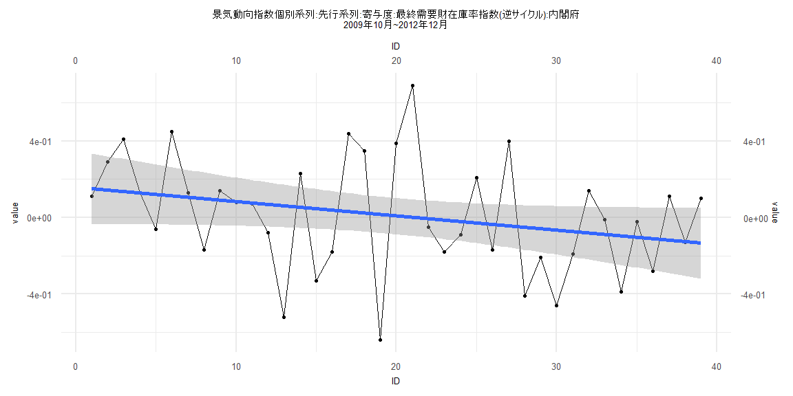
Call:
lm(formula = value ~ ID)

Residuals:
     Min       1Q   Median       3Q      Max
-0.65520 -0.16637 -0.00277  0.22618  0.68982

Coefficients:
             Estimate Std. Error t value Pr(>|t|)
(Intercept)  0.157854   0.095023   1.661   0.1051
ID          -0.007508   0.004141  -1.813   0.0779 .
---
Signif. codes:  0 '***' 0.001 '**' 0.01 '*' 0.05 '.' 0.1 ' ' 1

Residual standard error: 0.291 on 37 degrees of freedom
Multiple R-squared:  0.08161,   Adjusted R-squared:  0.05679
F-statistic: 3.288 on 1 and 37 DF,  p-value: 0.0779


    Two-sample Kolmogorov-Smirnov test

data:  lm_residuals and rnorm(n = length(lm_residuals), mean = 0, sd = sd(lm_residuals))
D = 0.12821, p-value = 0.9114
alternative hypothesis: two-sided


    Durbin-Watson test

data:  value ~ ID
DW = 2.253, p-value = 0.735
alternative hypothesis: true autocorrelation is greater than 0


    studentized Breusch-Pagan test

data:  value ~ ID
BP = 0.00073433, df = 1, p-value = 0.9784


    Box-Ljung test

data:  lm_residuals
X-squared = 0.77346, df = 1, p-value = 0.3791
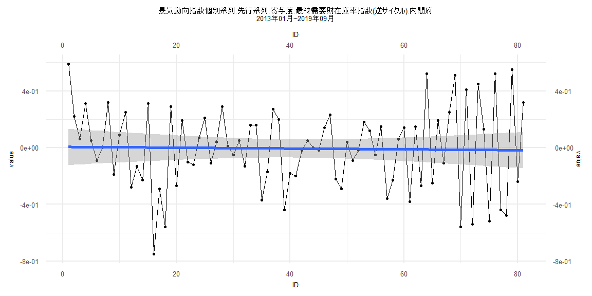
Call:
lm(formula = value ~ ID)

Residuals:
    Min      1Q  Median      3Q     Max
-0.7511 -0.2118  0.0127  0.2034  0.5846

Coefficients:
              Estimate Std. Error t value Pr(>|t|)
(Intercept)  0.0056975  0.0655884   0.087    0.931
ID          -0.0002895  0.0013896  -0.208    0.835

Residual standard error: 0.2924 on 79 degrees of freedom
Multiple R-squared:  0.0005492, Adjusted R-squared:  -0.0121
F-statistic: 0.04341 on 1 and 79 DF,  p-value: 0.8355


    Two-sample Kolmogorov-Smirnov test

data:  lm_residuals and rnorm(n = length(lm_residuals), mean = 0, sd = sd(lm_residuals))
D = 0.11111, p-value = 0.7027
alternative hypothesis: two-sided


    Durbin-Watson test

data:  value ~ ID
DW = 2.575, p-value = 0.9944
alternative hypothesis: true autocorrelation is greater than 0


    studentized Breusch-Pagan test

data:  value ~ ID
BP = 4.2385, df = 1, p-value = 0.03952


    Box-Ljung test

data:  lm_residuals
X-squared = 8.6726, df = 1, p-value = 0.00323
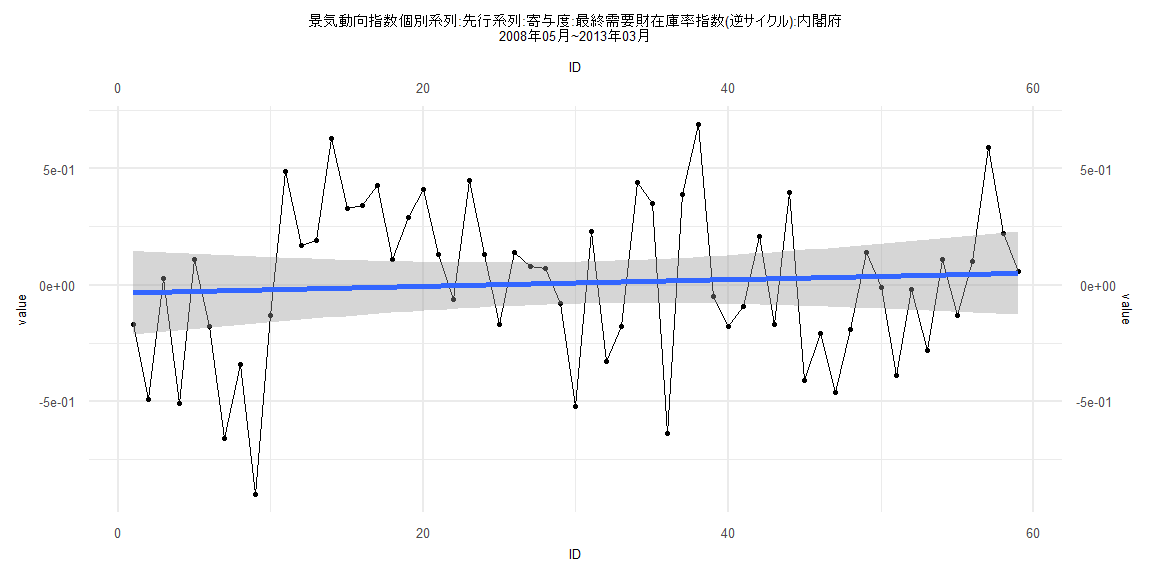
Call:
lm(formula = value ~ ID)

Residuals:
     Min       1Q   Median       3Q      Max
-0.87834 -0.20024  0.05384  0.21290  0.66981

Coefficients:
             Estimate Std. Error t value Pr(>|t|)
(Intercept) -0.034646   0.091346  -0.379    0.706
ID           0.001443   0.002648   0.545    0.588

Residual standard error: 0.3464 on 57 degrees of freedom
Multiple R-squared:  0.005183,  Adjusted R-squared:  -0.01227
F-statistic: 0.297 on 1 and 57 DF,  p-value: 0.5879


    Two-sample Kolmogorov-Smirnov test

data:  lm_residuals and rnorm(n = length(lm_residuals), mean = 0, sd = sd(lm_residuals))
D = 0.15254, p-value = 0.5021
alternative hypothesis: two-sided


    Durbin-Watson test

data:  value ~ ID
DW = 1.5667, p-value = 0.03354
alternative hypothesis: true autocorrelation is greater than 0


    studentized Breusch-Pagan test

data:  value ~ ID
BP = 2.1022, df = 1, p-value = 0.1471


    Box-Ljung test

data:  lm_residuals
X-squared = 2.8758, df = 1, p-value = 0.08992
Call:
lm(formula = value ~ ID)

Residuals:
     Min       1Q   Median       3Q      Max
-0.71656 -0.20314  0.02616  0.19293  0.54569

Coefficients:
              Estimate Std. Error t value Pr(>|t|)
(Intercept) -0.0412354  0.0659552  -0.625    0.534
ID           0.0005993  0.0014506   0.413    0.681

Residual standard error: 0.2885 on 76 degrees of freedom
Multiple R-squared:  0.00224,   Adjusted R-squared:  -0.01089
F-statistic: 0.1707 on 1 and 76 DF,  p-value: 0.6807


    Two-sample Kolmogorov-Smirnov test

data:  lm_residuals and rnorm(n = length(lm_residuals), mean = 0, sd = sd(lm_residuals))
D = 0.12821, p-value = 0.546
alternative hypothesis: two-sided


    Durbin-Watson test

data:  value ~ ID
DW = 2.7152, p-value = 0.9992
alternative hypothesis: true autocorrelation is greater than 0


    studentized Breusch-Pagan test

data:  value ~ ID
BP = 6.7838, df = 1, p-value = 0.009199


    Box-Ljung test

data:  lm_residuals
X-squared = 11.405, df = 1, p-value = 0.0007326