Analysis
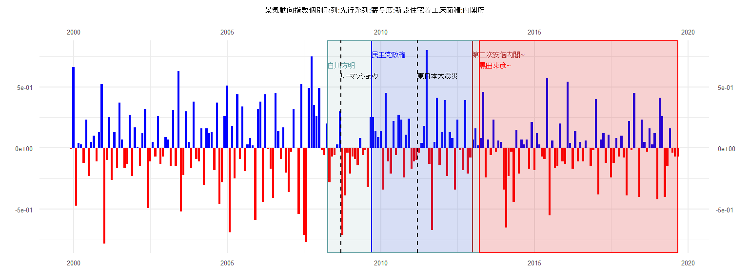
[1] "景気動向指数個別系列:先行系列:寄与度:新設住宅着工床面積:内閣府"
       Jan   Feb   Mar   Apr   May   Jun   Jul   Aug   Sep   Oct   Nov   Dec
1999                                                                   -0.01
2000  0.66 -0.47  0.04  0.03 -0.12  0.23 -0.23  0.05  0.10 -0.11  0.13  0.52
2001 -0.78 -0.10  0.25 -0.26  0.13 -0.16  0.37  0.07 -0.16 -0.13  0.27 -0.23
2002  0.17  0.01 -0.15  0.12  0.32 -0.49 -0.11  0.05 -0.07  0.26 -0.13 -0.07
2003  0.09  0.07 -0.15  0.31 -0.15  0.63 -0.52 -0.22  0.30  0.05 -0.16  0.38
2004 -0.09 -0.11  0.16 -0.30  0.16  0.12  0.13 -0.18  0.37 -0.46 -0.28  0.26
2005  0.51 -0.69  0.18 -0.25  0.44 -0.09  0.34 -0.19  0.03  0.08  0.02 -0.59
2006  0.32  0.38 -0.44  0.44 -0.01 -0.17 -0.41  0.45  0.14 -0.09  0.17 -0.20
2007 -0.36 -0.03  0.32  0.00 -0.54  0.52 -0.71 -0.77  0.49  0.75  0.35  0.26
2008  0.49 -0.02 -0.06  0.20 -0.28 -0.07 -0.06  0.03  0.30 -0.71 -0.39 -0.04
2009 -0.21 -0.07 -0.09 -0.14  0.08 -0.06 -0.02 -0.32  0.25  0.25  0.14  0.09
2010  0.14 -0.34  0.45 -0.11 -0.21  0.22 -0.06  0.27  0.23 -0.24  0.11  0.24
2011 -0.17 -0.11 -0.10 -0.04  0.04  0.18  0.80 -0.13 -0.67  0.05  0.41 -0.14
2012  0.13  0.39 -0.23  0.13  0.08 -0.34  0.23 -0.02 -0.18  0.39 -0.21 -0.08
2013  0.07  0.16  0.02  0.08  0.46 -0.24  0.07 -0.06  0.23 -0.03  0.06  0.05
2014 -0.34 -0.65 -0.23 -0.03 -0.44  0.15 -0.21  0.07  0.03  0.07 -0.17  0.21
2015 -0.18  0.12  0.03 -0.07 -0.09  0.57 -0.55  0.06 -0.16 -0.15  0.20 -0.11
2016 -0.13  0.54  0.04 -0.17  0.14 -0.11  0.05 -0.11  0.06  0.00 -0.15 -0.02
2017  0.40 -0.38  0.07  0.12 -0.12  0.11 -0.24 -0.12  0.08 -0.07  0.10 -0.08
2018 -0.39  0.22 -0.02  0.45  0.00 -0.40  0.23  0.05 -0.03  0.16  0.03  0.12
2019 -0.42  0.41  0.26 -0.40 -0.15  0.16 -0.04 -0.07 -0.07
Call:
lm(formula = value ~ ID)

Residuals:
     Min       1Q   Median       3Q      Max
-0.70164 -0.17262  0.01041  0.15998  0.76380

Coefficients:
             Estimate Std. Error t value Pr(>|t|)
(Intercept)  0.086437   0.088697   0.975    0.336
ID          -0.002283   0.003865  -0.591    0.558

Residual standard error: 0.2716 on 37 degrees of freedom
Multiple R-squared:  0.009345,  Adjusted R-squared:  -0.01743
F-statistic: 0.349 on 1 and 37 DF,  p-value: 0.5582


    Two-sample Kolmogorov-Smirnov test

data:  lm_residuals and rnorm(n = length(lm_residuals), mean = 0, sd = sd(lm_residuals))
D = 0.12821, p-value = 0.9114
alternative hypothesis: two-sided


    Durbin-Watson test

data:  value ~ ID
DW = 2.4059, p-value = 0.8686
alternative hypothesis: true autocorrelation is greater than 0


    studentized Breusch-Pagan test

data:  value ~ ID
BP = 0.22823, df = 1, p-value = 0.6328


    Box-Ljung test

data:  lm_residuals
X-squared = 1.8399, df = 1, p-value = 0.175
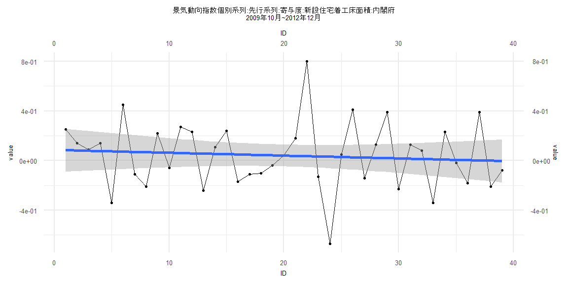
Call:
lm(formula = value ~ ID)

Residuals:
     Min       1Q   Median       3Q      Max
-0.63330 -0.11817  0.00993  0.11824  0.58332

Coefficients:
              Estimate Std. Error t value Pr(>|t|)
(Intercept) -0.0196636  0.0519916  -0.378    0.706
ID           0.0002116  0.0011016   0.192    0.848

Residual standard error: 0.2318 on 79 degrees of freedom
Multiple R-squared:  0.0004669, Adjusted R-squared:  -0.01219
F-statistic: 0.0369 on 1 and 79 DF,  p-value: 0.8482


    Two-sample Kolmogorov-Smirnov test

data:  lm_residuals and rnorm(n = length(lm_residuals), mean = 0, sd = sd(lm_residuals))
D = 0.12346, p-value = 0.5705
alternative hypothesis: two-sided


    Durbin-Watson test

data:  value ~ ID
DW = 2.4861, p-value = 0.9827
alternative hypothesis: true autocorrelation is greater than 0


    studentized Breusch-Pagan test

data:  value ~ ID
BP = 0.063588, df = 1, p-value = 0.8009


    Box-Ljung test

data:  lm_residuals
X-squared = 5.0241, df = 1, p-value = 0.025
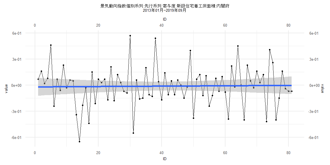
Call:
lm(formula = value ~ ID)

Residuals:
     Min       1Q   Median       3Q      Max
-0.70172 -0.15647  0.00833  0.16073  0.77393

Coefficients:
             Estimate Std. Error t value Pr(>|t|)
(Intercept) -0.083974   0.068121  -1.233    0.223
ID           0.002822   0.001975   1.429    0.158

Residual standard error: 0.2583 on 57 degrees of freedom
Multiple R-squared:  0.03458,   Adjusted R-squared:  0.01765
F-statistic: 2.042 on 1 and 57 DF,  p-value: 0.1585


    Two-sample Kolmogorov-Smirnov test

data:  lm_residuals and rnorm(n = length(lm_residuals), mean = 0, sd = sd(lm_residuals))
D = 0.13559, p-value = 0.6544
alternative hypothesis: two-sided


    Durbin-Watson test

data:  value ~ ID
DW = 2.2417, p-value = 0.7881
alternative hypothesis: true autocorrelation is greater than 0


    studentized Breusch-Pagan test

data:  value ~ ID
BP = 0.041041, df = 1, p-value = 0.8395


    Box-Ljung test

data:  lm_residuals
X-squared = 0.99368, df = 1, p-value = 0.3188
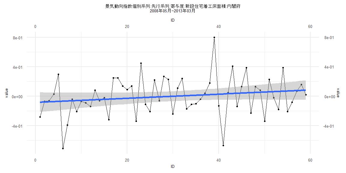
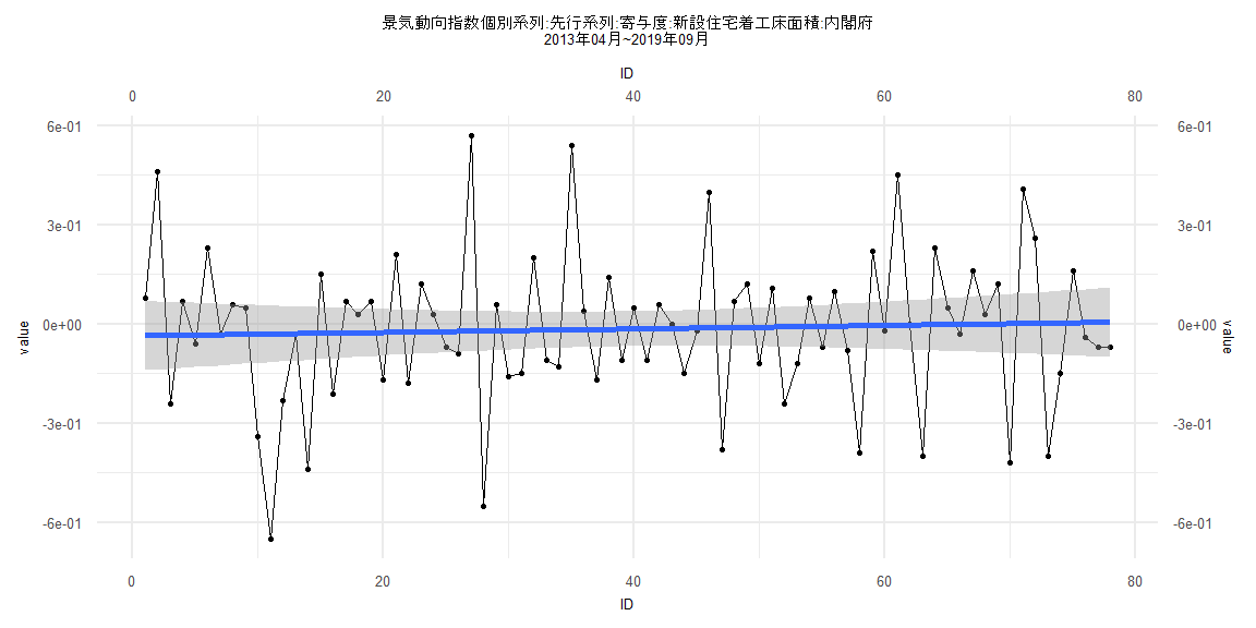
Call:
lm(formula = value ~ ID)

Residuals:
     Min       1Q   Median       3Q      Max
-0.62033 -0.12630  0.00226  0.11764  0.59122

Coefficients:
              Estimate Std. Error t value Pr(>|t|)
(Intercept) -0.0354745  0.0537381  -0.660    0.511
ID           0.0005281  0.0011819   0.447    0.656

Residual standard error: 0.235 on 76 degrees of freedom
Multiple R-squared:  0.00262,   Adjusted R-squared:  -0.0105
F-statistic: 0.1996 on 1 and 76 DF,  p-value: 0.6563


    Two-sample Kolmogorov-Smirnov test

data:  lm_residuals and rnorm(n = length(lm_residuals), mean = 0, sd = sd(lm_residuals))
D = 0.11538, p-value = 0.6802
alternative hypothesis: two-sided


    Durbin-Watson test

data:  value ~ ID
DW = 2.5064, p-value = 0.9848
alternative hypothesis: true autocorrelation is greater than 0


    studentized Breusch-Pagan test

data:  value ~ ID
BP = 0.28198, df = 1, p-value = 0.5954


    Box-Ljung test

data:  lm_residuals
X-squared = 5.2876, df = 1, p-value = 0.02148