Analysis
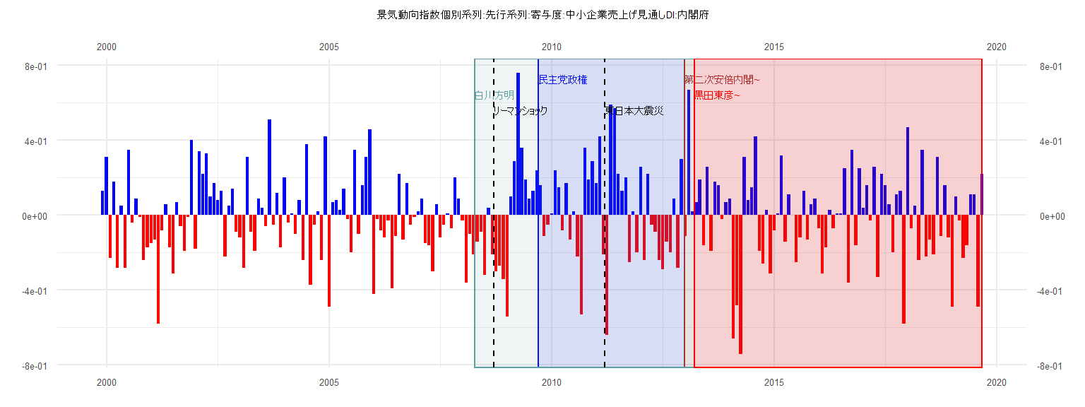
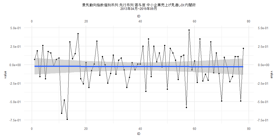
[1] "景気動向指数個別系列:先行系列:寄与度:中小企業売上げ見通しDI:内閣府"
       Jan   Feb   Mar   Apr   May   Jun   Jul   Aug   Sep   Oct   Nov   Dec
1999                                                                    0.13
2000  0.31 -0.23  0.18 -0.28  0.05 -0.28  0.35 -0.04  0.09 -0.01 -0.24 -0.17
2001 -0.15 -0.13 -0.58 -0.08  0.06 -0.17 -0.31  0.07 -0.06 -0.19 -0.01  0.40
2002 -0.18  0.34  0.22  0.33  0.10  0.17  0.08  0.13 -0.22  0.05  0.14 -0.09
2003 -0.12 -0.28  0.31 -0.09 -0.19  0.09  0.04 -0.06  0.51 -0.05  0.12 -0.17
2004  0.20 -0.04  0.01 -0.10  0.08 -0.24  0.38 -0.37 -0.05  0.02 -0.24  0.42
2005 -0.49  0.07  0.08  0.03  0.14 -0.02 -0.20  0.35 -0.10  0.16  0.31  0.46
2006 -0.42 -0.02 -0.08 -0.12 -0.03 -0.39 -0.11  0.22 -0.13  0.17 -0.05 -0.01
2007  0.02  0.09 -0.15 -0.16 -0.30  0.06 -0.12 -0.05  0.01 -0.07  0.20  0.09
2008 -0.03 -0.36 -0.10 -0.21 -0.14 -0.09 -0.32  0.04 -0.21 -0.30 -0.27 -0.34
2009 -0.54  0.10  0.29  0.76  0.36  0.19  0.09  0.13  0.24  0.16 -0.11 -0.05
2010  0.01  0.24  0.15 -0.08  0.17 -0.13  0.02 -0.22 -0.53  0.36  0.19  0.29
2011  0.17  0.42 -0.21 -0.64  0.59  0.57  0.22  0.13  0.20 -0.25  0.02 -0.20
2012  0.26 -0.24  0.22 -0.05 -0.09 -0.24 -0.29 -0.14 -0.20  0.09 -0.28  0.30
2013 -0.11  0.67  0.02  0.07  0.19 -0.16  0.26 -0.19  0.18  0.16 -0.02  0.07
2014  0.09 -0.66 -0.48 -0.74  0.31  0.08  0.15  0.42 -0.19 -0.26  0.03 -0.31
2015 -0.08  0.01  0.32 -0.14  0.11  0.00 -0.25 -0.12  0.13 -0.13  0.06  0.09
2016 -0.07 -0.31 -0.17  0.03 -0.07  0.01  0.01  0.25 -0.36  0.35 -0.16  0.25
2017  0.04  0.16 -0.03  0.26 -0.33  0.22  0.16  0.06 -0.20  0.11  0.13 -0.58
2018  0.47 -0.07  0.05 -0.24  0.35 -0.22 -0.13 -0.21  0.31 -0.11  0.16 -0.12
2019 -0.49  0.10 -0.03 -0.23 -0.16  0.11  0.11 -0.49  0.22
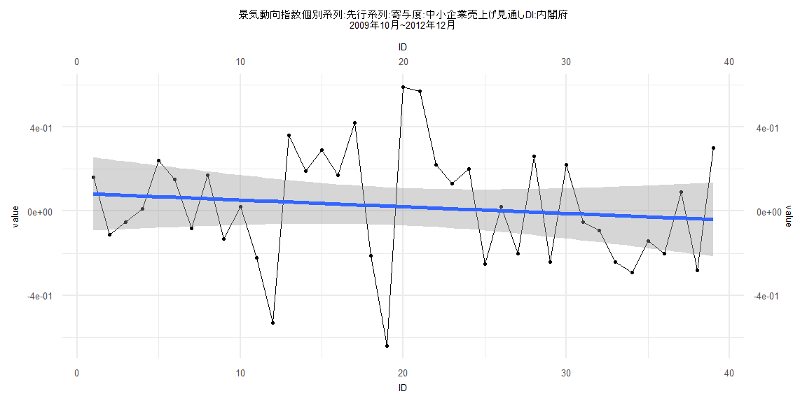
Call:
lm(formula = value ~ ID)

Residuals:
     Min       1Q   Median       3Q      Max
-0.66447 -0.19381 -0.03314  0.18119  0.56872

Coefficients:
             Estimate Std. Error t value Pr(>|t|)
(Intercept)  0.085007   0.089605   0.949    0.349
ID          -0.003186   0.003904  -0.816    0.420

Residual standard error: 0.2744 on 37 degrees of freedom
Multiple R-squared:  0.01768,   Adjusted R-squared:  -0.008869
F-statistic: 0.6659 on 1 and 37 DF,  p-value: 0.4197


    Two-sample Kolmogorov-Smirnov test

data:  lm_residuals and rnorm(n = length(lm_residuals), mean = 0, sd = sd(lm_residuals))
D = 0.15385, p-value = 0.7523
alternative hypothesis: two-sided


    Durbin-Watson test

data:  value ~ ID
DW = 1.9173, p-value = 0.3324
alternative hypothesis: true autocorrelation is greater than 0


    studentized Breusch-Pagan test

data:  value ~ ID
BP = 0.008385, df = 1, p-value = 0.927


    Box-Ljung test

data:  lm_residuals
X-squared = 0.016181, df = 1, p-value = 0.8988
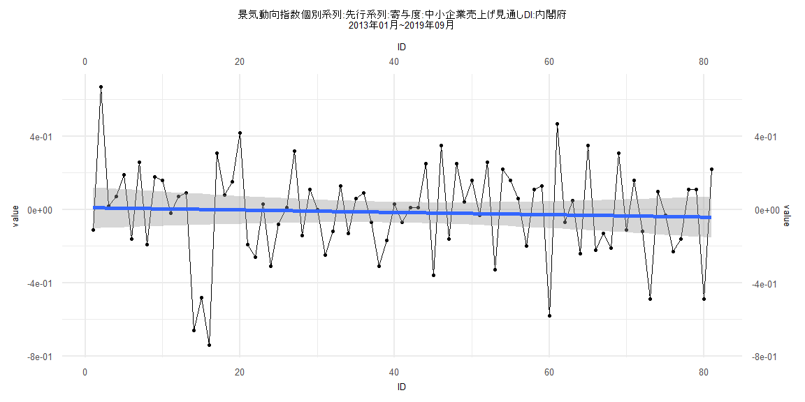
Call:
lm(formula = value ~ ID)

Residuals:
     Min       1Q   Median       3Q      Max
-0.74028 -0.15548  0.02645  0.15586  0.66071

Coefficients:
              Estimate Std. Error t value Pr(>|t|)
(Intercept)  0.0105772  0.0574214   0.184    0.854
ID          -0.0006434  0.0012166  -0.529    0.598

Residual standard error: 0.256 on 79 degrees of freedom
Multiple R-squared:  0.003528,  Adjusted R-squared:  -0.009086
F-statistic: 0.2797 on 1 and 79 DF,  p-value: 0.5984


    Two-sample Kolmogorov-Smirnov test

data:  lm_residuals and rnorm(n = length(lm_residuals), mean = 0, sd = sd(lm_residuals))
D = 0.08642, p-value = 0.9254
alternative hypothesis: two-sided


    Durbin-Watson test

data:  value ~ ID
DW = 2.3533, p-value = 0.9323
alternative hypothesis: true autocorrelation is greater than 0


    studentized Breusch-Pagan test

data:  value ~ ID
BP = 0.87395, df = 1, p-value = 0.3499


    Box-Ljung test

data:  lm_residuals
X-squared = 2.8646, df = 1, p-value = 0.09055
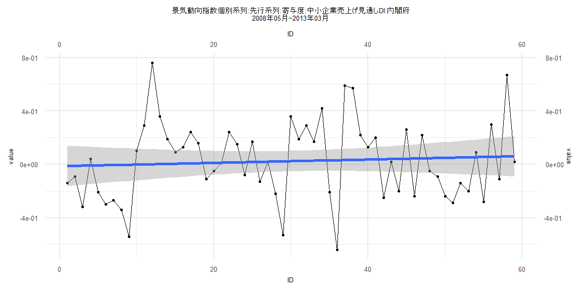
Call:
lm(formula = value ~ ID)

Residuals:
     Min       1Q   Median       3Q      Max
-0.67125 -0.24061 -0.00244  0.17997  0.75885

Coefficients:
             Estimate Std. Error t value Pr(>|t|)
(Intercept) -0.013898   0.077492  -0.179    0.858
ID           0.001254   0.002246   0.558    0.579

Residual standard error: 0.2938 on 57 degrees of freedom
Multiple R-squared:  0.005439,  Adjusted R-squared:  -0.01201
F-statistic: 0.3117 on 1 and 57 DF,  p-value: 0.5788


    Two-sample Kolmogorov-Smirnov test

data:  lm_residuals and rnorm(n = length(lm_residuals), mean = 0, sd = sd(lm_residuals))
D = 0.10169, p-value = 0.9239
alternative hypothesis: two-sided


    Durbin-Watson test

data:  value ~ ID
DW = 1.57, p-value = 0.03456
alternative hypothesis: true autocorrelation is greater than 0


    studentized Breusch-Pagan test

data:  value ~ ID
BP = 0.012466, df = 1, p-value = 0.9111


    Box-Ljung test

data:  lm_residuals
X-squared = 2.8197, df = 1, p-value = 0.09311
Call:
lm(formula = value ~ ID)

Residuals:
     Min       1Q   Median       3Q      Max
-0.71831 -0.14461  0.03385  0.16775  0.49535

Coefficients:
               Estimate  Std. Error t value Pr(>|t|)
(Intercept) -0.02063936  0.05692255  -0.363    0.718
ID          -0.00008118  0.00125198  -0.065    0.948

Residual standard error: 0.249 on 76 degrees of freedom
Multiple R-squared:  5.532e-05, Adjusted R-squared:  -0.0131
F-statistic: 0.004205 on 1 and 76 DF,  p-value: 0.9485


    Two-sample Kolmogorov-Smirnov test

data:  lm_residuals and rnorm(n = length(lm_residuals), mean = 0, sd = sd(lm_residuals))
D = 0.16667, p-value = 0.2297
alternative hypothesis: two-sided


    Durbin-Watson test

data:  value ~ ID
DW = 2.3673, p-value = 0.9363
alternative hypothesis: true autocorrelation is greater than 0


    studentized Breusch-Pagan test

data:  value ~ ID
BP = 0.23457, df = 1, p-value = 0.6282


    Box-Ljung test

data:  lm_residuals
X-squared = 2.9567, df = 1, p-value = 0.08552