Analysis
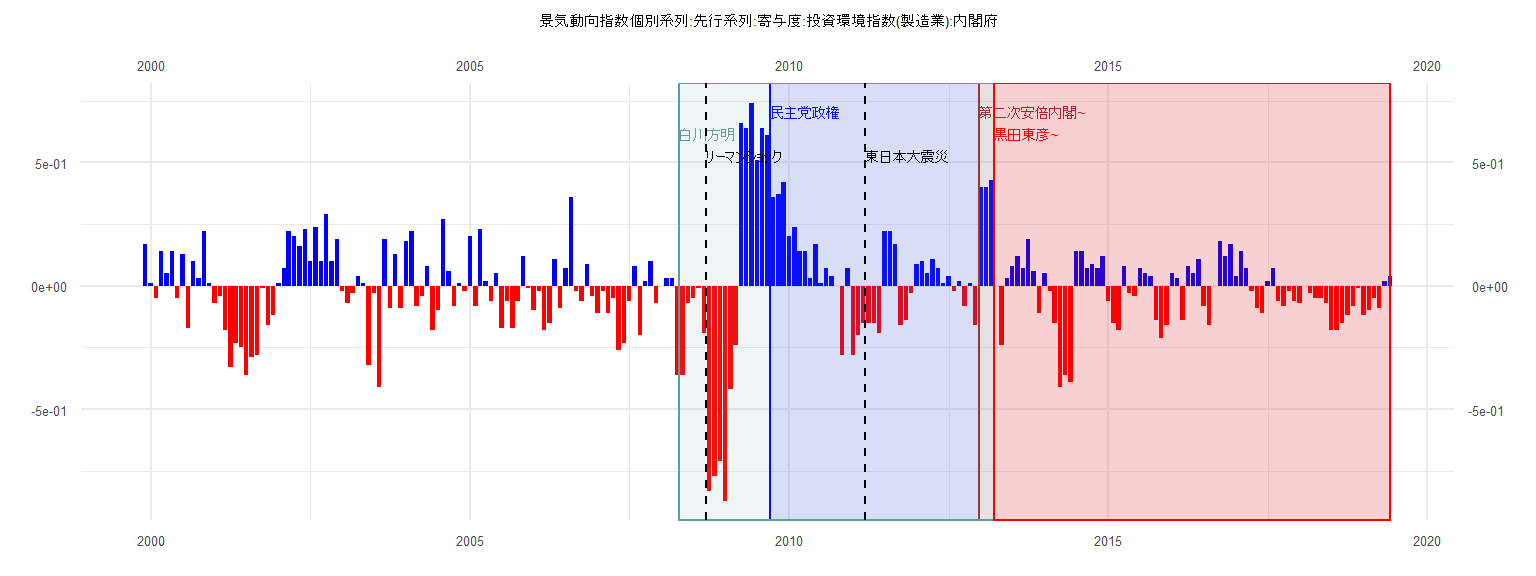
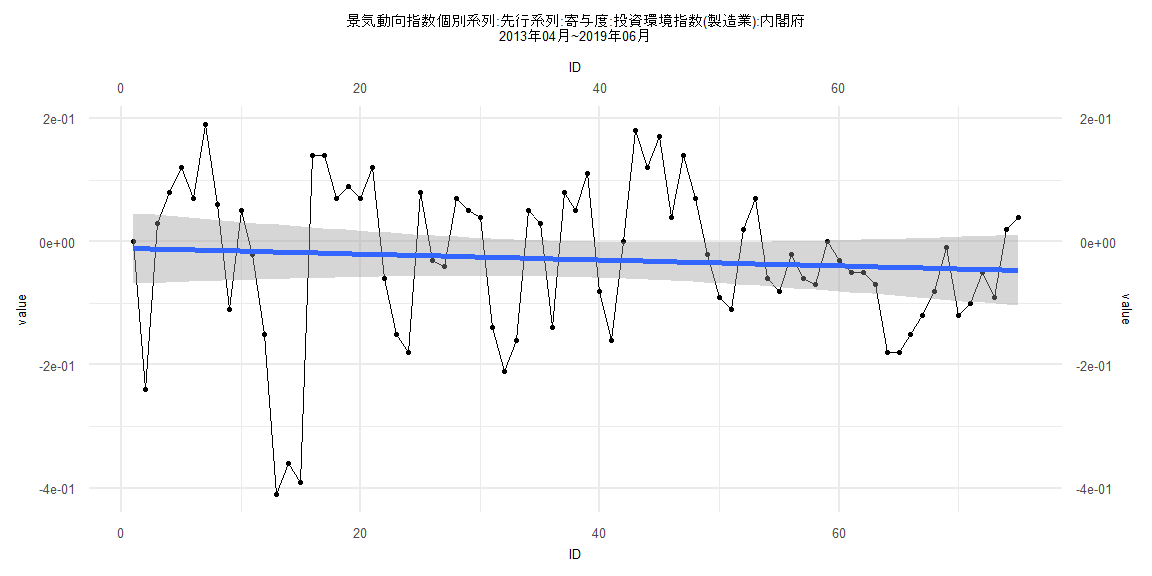
[1] "景気動向指数個別系列:先行系列:寄与度:投資環境指数(製造業):内閣府"
       Jan   Feb   Mar   Apr   May   Jun   Jul   Aug   Sep   Oct   Nov   Dec
1999                                                                    0.17
2000  0.01 -0.05  0.14  0.05  0.14 -0.05  0.13 -0.17  0.10  0.03  0.22  0.01
2001 -0.07 -0.04 -0.18 -0.33 -0.23 -0.25 -0.36 -0.29 -0.28 -0.01 -0.16 -0.12
2002  0.01  0.07  0.22  0.20  0.16  0.23  0.10  0.24  0.10  0.29  0.10  0.19
2003 -0.02 -0.07 -0.03  0.04  0.01 -0.32 -0.03 -0.41  0.19 -0.09  0.13 -0.09
2004  0.18  0.22 -0.08 -0.04  0.08 -0.18 -0.10  0.27  0.06 -0.08  0.01 -0.02
2005  0.20 -0.08  0.23  0.02 -0.06  0.05 -0.17 -0.06 -0.17 -0.06  0.12 -0.01
2006 -0.10 -0.02 -0.18 -0.15  0.11 -0.09  0.07  0.36 -0.02 -0.06  0.09 -0.04
2007 -0.11 -0.02 -0.11 -0.05 -0.26 -0.23 -0.06  0.08 -0.20  0.02  0.10 -0.07
2008  0.00  0.03  0.03 -0.36 -0.36 -0.07 -0.05 -0.01 -0.19 -0.83 -0.77 -0.71
2009 -0.87 -0.42 -0.24  0.66  0.64  0.74  0.51  0.64  0.61  0.36  0.37  0.42
2010  0.20  0.24  0.14  0.14  0.03  0.17  0.01  0.07  0.04  0.00 -0.28  0.07
2011 -0.28 -0.20 -0.15 -0.15 -0.15 -0.19  0.22  0.22  0.17 -0.16 -0.14 -0.03
2012  0.09  0.10  0.05  0.11  0.07  0.01  0.04 -0.02  0.02 -0.08  0.01 -0.16
2013  0.40  0.40  0.43  0.00 -0.24  0.03  0.08  0.12  0.07  0.19  0.06 -0.11
2014  0.05 -0.02 -0.15 -0.41 -0.36 -0.39  0.14  0.14  0.07  0.09  0.07  0.12
2015 -0.06 -0.15 -0.18  0.08 -0.03 -0.04  0.07  0.05  0.04 -0.14 -0.21 -0.16
2016  0.05  0.03 -0.14  0.08  0.05  0.11 -0.08 -0.16  0.00  0.18  0.12  0.17
2017  0.04  0.14  0.07 -0.02 -0.09 -0.11  0.02  0.07 -0.06 -0.08 -0.02 -0.06
2018 -0.07  0.00 -0.03 -0.05 -0.05 -0.07 -0.18 -0.18 -0.15 -0.12 -0.08 -0.01
2019 -0.12 -0.10 -0.05 -0.09  0.02  0.04
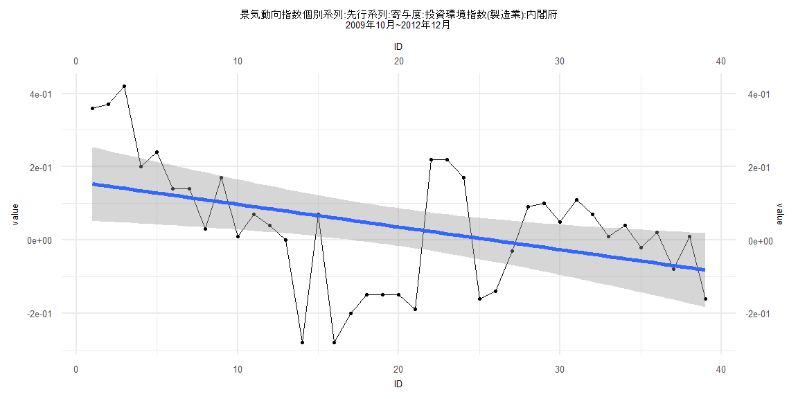
Call:
lm(formula = value ~ ID)

Residuals:
     Min       1Q   Median       3Q      Max
-0.35255 -0.08352  0.02409  0.10656  0.27931

Coefficients:
             Estimate Std. Error t value Pr(>|t|)
(Intercept)  0.159271   0.051683   3.082  0.00387 **
ID          -0.006194   0.002252  -2.751  0.00915 **
---
Signif. codes:  0 '***' 0.001 '**' 0.01 '*' 0.05 '.' 0.1 ' ' 1

Residual standard error: 0.1583 on 37 degrees of freedom
Multiple R-squared:  0.1698,    Adjusted R-squared:  0.1473
F-statistic: 7.565 on 1 and 37 DF,  p-value: 0.009154


    Two-sample Kolmogorov-Smirnov test

data:  lm_residuals and rnorm(n = length(lm_residuals), mean = 0, sd = sd(lm_residuals))
D = 0.10256, p-value = 0.9885
alternative hypothesis: two-sided


    Durbin-Watson test

data:  value ~ ID
DW = 0.89083, p-value = 0.00003079
alternative hypothesis: true autocorrelation is greater than 0


    studentized Breusch-Pagan test

data:  value ~ ID
BP = 2.5161, df = 1, p-value = 0.1127


    Box-Ljung test

data:  lm_residuals
X-squared = 11.741, df = 1, p-value = 0.0006112
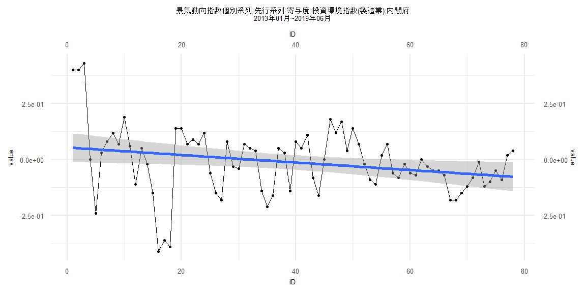
Call:
lm(formula = value ~ ID)

Residuals:
     Min       1Q   Median       3Q      Max
-0.43746 -0.05658  0.01933  0.07141  0.38075

Coefficients:
              Estimate Std. Error t value Pr(>|t|)
(Intercept)  0.0542757  0.0332771   1.631   0.1070
ID          -0.0016759  0.0007319  -2.290   0.0248 *
---
Signif. codes:  0 '***' 0.001 '**' 0.01 '*' 0.05 '.' 0.1 ' ' 1

Residual standard error: 0.1455 on 76 degrees of freedom
Multiple R-squared:  0.06454,   Adjusted R-squared:  0.05223
F-statistic: 5.243 on 1 and 76 DF,  p-value: 0.02481


    Two-sample Kolmogorov-Smirnov test

data:  lm_residuals and rnorm(n = length(lm_residuals), mean = 0, sd = sd(lm_residuals))
D = 0.12821, p-value = 0.546
alternative hypothesis: two-sided


    Durbin-Watson test

data:  value ~ ID
DW = 0.83206, p-value = 0.000000002444
alternative hypothesis: true autocorrelation is greater than 0


    studentized Breusch-Pagan test

data:  value ~ ID
BP = 13.681, df = 1, p-value = 0.0002167


    Box-Ljung test

data:  lm_residuals
X-squared = 23.83, df = 1, p-value = 0.000001052
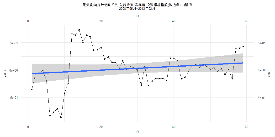
Call:
lm(formula = value ~ ID)

Residuals:
     Min       1Q   Median       3Q      Max
-0.83130 -0.20393 -0.00772  0.15597  0.76186

Coefficients:
             Estimate Std. Error t value Pr(>|t|)
(Intercept) -0.069012   0.091091  -0.758    0.452
ID           0.003368   0.002641   1.276    0.207

Residual standard error: 0.3454 on 57 degrees of freedom
Multiple R-squared:  0.02775,   Adjusted R-squared:  0.0107
F-statistic: 1.627 on 1 and 57 DF,  p-value: 0.2073


    Two-sample Kolmogorov-Smirnov test

data:  lm_residuals and rnorm(n = length(lm_residuals), mean = 0, sd = sd(lm_residuals))
D = 0.18644, p-value = 0.2582
alternative hypothesis: two-sided


    Durbin-Watson test

data:  value ~ ID
DW = 0.42499, p-value = 0.0000000000000041
alternative hypothesis: true autocorrelation is greater than 0


    studentized Breusch-Pagan test

data:  value ~ ID
BP = 14.758, df = 1, p-value = 0.0001222


    Box-Ljung test

data:  lm_residuals
X-squared = 37.222, df = 1, p-value = 0.000000001054
Call:
lm(formula = value ~ ID)

Residuals:
     Min       1Q   Median       3Q      Max
-0.39324 -0.06518  0.01098  0.08789  0.21121

Coefficients:
              Estimate Std. Error t value Pr(>|t|)
(Intercept) -0.0104973  0.0293626  -0.358    0.722
ID          -0.0004817  0.0006714  -0.717    0.475

Residual standard error: 0.1259 on 73 degrees of freedom
Multiple R-squared:  0.007001,  Adjusted R-squared:  -0.006602
F-statistic: 0.5147 on 1 and 73 DF,  p-value: 0.4754


    Two-sample Kolmogorov-Smirnov test

data:  lm_residuals and rnorm(n = length(lm_residuals), mean = 0, sd = sd(lm_residuals))
D = 0.14667, p-value = 0.3974
alternative hypothesis: two-sided


    Durbin-Watson test

data:  value ~ ID
DW = 0.99829, p-value = 0.0000007995
alternative hypothesis: true autocorrelation is greater than 0


    studentized Breusch-Pagan test

data:  value ~ ID
BP = 8.002, df = 1, p-value = 0.004673


    Box-Ljung test

data:  lm_residuals
X-squared = 19.32, df = 1, p-value = 0.00001105