Analysis
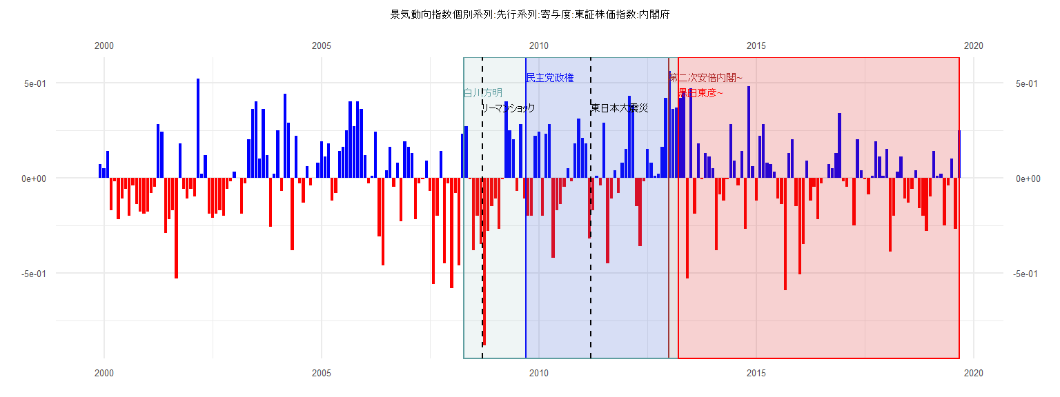
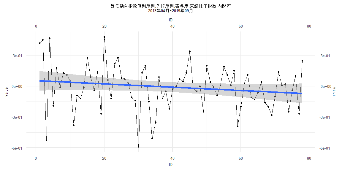
[1] "景気動向指数個別系列:先行系列:寄与度:東証株価指数:内閣府"
       Jan   Feb   Mar   Apr   May   Jun   Jul   Aug   Sep   Oct   Nov   Dec
1999                                                                    0.07
2000  0.05  0.14 -0.17 -0.02 -0.22 -0.11 -0.06 -0.20 -0.04 -0.14 -0.18 -0.19
2001 -0.18 -0.08 -0.05  0.28  0.24 -0.29 -0.22 -0.17 -0.53  0.18 -0.06 -0.11
2002 -0.06 -0.10  0.52  0.02  0.12 -0.19 -0.21 -0.19 -0.17 -0.20 -0.06 -0.02
2003  0.03  0.00 -0.19 -0.03  0.20  0.36  0.40  0.10  0.36  0.12 -0.26  0.02
2004  0.25 -0.07  0.44  0.29 -0.38  0.22 -0.03 -0.13  0.06 -0.04  0.00  0.08
2005  0.19  0.11  0.18 -0.12 -0.08  0.14  0.16  0.25  0.40  0.27  0.40  0.36
2006  0.12 -0.03  0.01  0.24 -0.31 -0.46  0.04  0.16 -0.05  0.08 -0.23  0.19
2007  0.16  0.13 -0.22 -0.03 -0.01  0.09 -0.07 -0.56 -0.20  0.14 -0.45 -0.03
2008 -0.58 -0.08 -0.46  0.23  0.27 -0.01 -0.38 -0.20 -0.35 -0.88 -0.28 -0.15
2009 -0.11 -0.27 -0.01  0.40  0.25  0.20 -0.07  0.28 -0.11 -0.20 -0.20  0.22
2010  0.24 -0.20  0.23  0.28 -0.42 -0.17 -0.14 -0.05  0.05 -0.02  0.18  0.31
2011  0.21  0.18 -0.32 -0.17  0.01 -0.04  0.29 -0.45 -0.11  0.04 -0.08  0.08
2012  0.15  0.43  0.38 -0.15 -0.36 -0.02  0.15  0.08  0.01  0.02  0.16  0.42
2013  0.56  0.36  0.37  0.42  0.45 -0.53  0.47 -0.19  0.18 -0.01  0.13  0.11
2014  0.05 -0.38 -0.09 -0.12 -0.01  0.28  0.09 -0.04  0.14 -0.27  0.48  0.06
2015 -0.12  0.22  0.28  0.08  0.07  0.03 -0.11 -0.14 -0.59  0.13  0.20 -0.15
2016 -0.51 -0.35  0.09 -0.12 -0.05 -0.22 -0.03  0.00  0.07  0.05  0.13  0.34
2017 -0.02 -0.05  0.00 -0.25  0.20  0.04 -0.01 -0.09  0.01  0.19  0.11  0.01
2018  0.15 -0.39 -0.20  0.03  0.11 -0.11 -0.13 -0.06  0.04 -0.16 -0.20 -0.28
2019 -0.10  0.14  0.01  0.02 -0.25 -0.04  0.10 -0.27  0.25
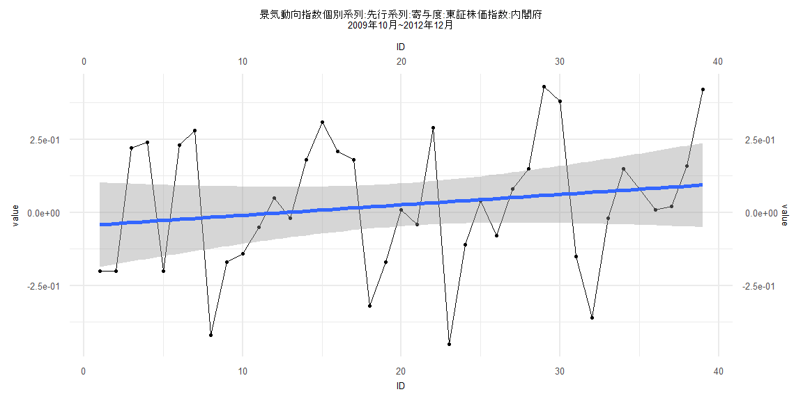
Call:
lm(formula = value ~ ID)

Residuals:
     Min       1Q   Median       3Q      Max
-0.48684 -0.15369 -0.01615  0.18665  0.37180

Coefficients:
             Estimate Std. Error t value Pr(>|t|)
(Intercept) -0.045061   0.073700  -0.611    0.545
ID           0.003561   0.003211   1.109    0.275

Residual standard error: 0.2257 on 37 degrees of freedom
Multiple R-squared:  0.03216,   Adjusted R-squared:  0.005999
F-statistic: 1.229 on 1 and 37 DF,  p-value: 0.2747


    Two-sample Kolmogorov-Smirnov test

data:  lm_residuals and rnorm(n = length(lm_residuals), mean = 0, sd = sd(lm_residuals))
D = 0.17949, p-value = 0.5622
alternative hypothesis: two-sided


    Durbin-Watson test

data:  value ~ ID
DW = 1.5874, p-value = 0.06837
alternative hypothesis: true autocorrelation is greater than 0


    studentized Breusch-Pagan test

data:  value ~ ID
BP = 0.03834, df = 1, p-value = 0.8448


    Box-Ljung test

data:  lm_residuals
X-squared = 1.2361, df = 1, p-value = 0.2662
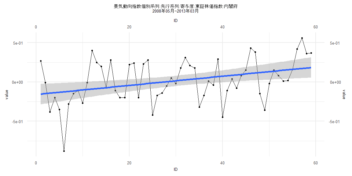
Call:
lm(formula = value ~ ID)

Residuals:
     Min       1Q   Median       3Q      Max
-0.62850 -0.13013  0.01886  0.13806  0.44850

Coefficients:
             Estimate Std. Error t value Pr(>|t|)
(Intercept)  0.114096   0.049561   2.302   0.0240 *
ID          -0.002599   0.001050  -2.475   0.0155 *
---
Signif. codes:  0 '***' 0.001 '**' 0.01 '*' 0.05 '.' 0.1 ' ' 1

Residual standard error: 0.221 on 79 degrees of freedom
Multiple R-squared:  0.07197,   Adjusted R-squared:  0.06022
F-statistic: 6.127 on 1 and 79 DF,  p-value: 0.01546


    Two-sample Kolmogorov-Smirnov test

data:  lm_residuals and rnorm(n = length(lm_residuals), mean = 0, sd = sd(lm_residuals))
D = 0.14815, p-value = 0.338
alternative hypothesis: two-sided


    Durbin-Watson test

data:  value ~ ID
DW = 1.8759, p-value = 0.2494
alternative hypothesis: true autocorrelation is greater than 0


    studentized Breusch-Pagan test

data:  value ~ ID
BP = 7.0145, df = 1, p-value = 0.008085


    Box-Ljung test

data:  lm_residuals
X-squared = 0.035048, df = 1, p-value = 0.8515
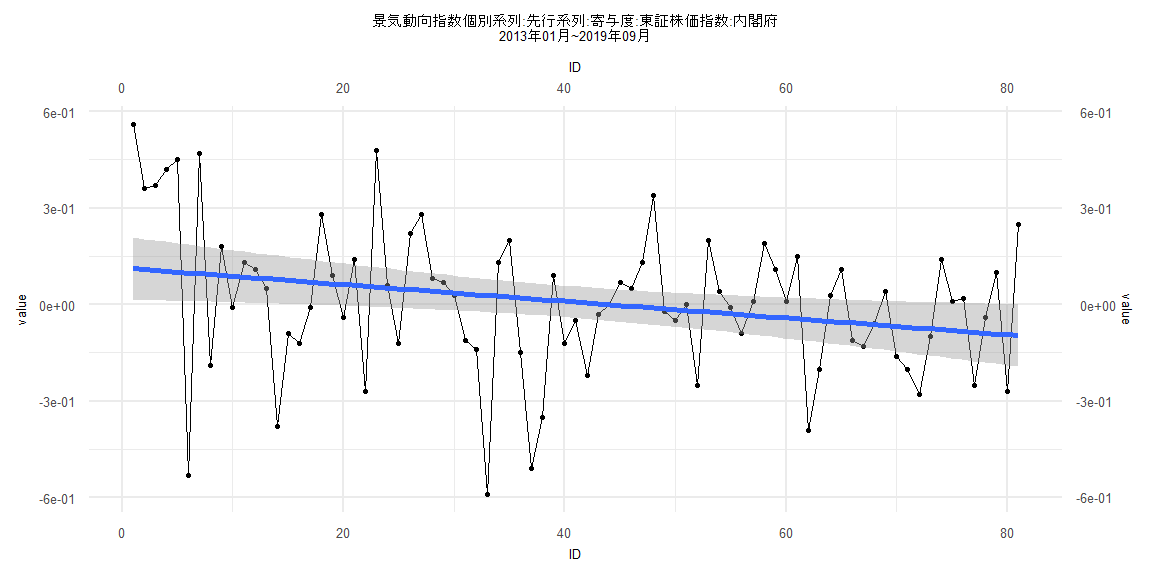
Call:
lm(formula = value ~ ID)

Residuals:
     Min       1Q   Median       3Q      Max
-0.75483 -0.15632 -0.03508  0.20388  0.49011

Coefficients:
             Estimate Std. Error t value Pr(>|t|)
(Intercept) -0.160234   0.066781  -2.399  0.01971 *
ID           0.005844   0.001936   3.019  0.00379 **
---
Signif. codes:  0 '***' 0.001 '**' 0.01 '*' 0.05 '.' 0.1 ' ' 1

Residual standard error: 0.2532 on 57 degrees of freedom
Multiple R-squared:  0.1378,    Adjusted R-squared:  0.1227
F-statistic: 9.113 on 1 and 57 DF,  p-value: 0.003792


    Two-sample Kolmogorov-Smirnov test

data:  lm_residuals and rnorm(n = length(lm_residuals), mean = 0, sd = sd(lm_residuals))
D = 0.11864, p-value = 0.8052
alternative hypothesis: two-sided


    Durbin-Watson test

data:  value ~ ID
DW = 1.2663, p-value = 0.00105
alternative hypothesis: true autocorrelation is greater than 0


    studentized Breusch-Pagan test

data:  value ~ ID
BP = 1.3045, df = 1, p-value = 0.2534


    Box-Ljung test

data:  lm_residuals
X-squared = 7.0674, df = 1, p-value = 0.00785
Call:
lm(formula = value ~ ID)

Residuals:
    Min      1Q  Median      3Q     Max
-0.5966 -0.1241  0.0206  0.1223  0.4574

Coefficients:
             Estimate Std. Error t value Pr(>|t|)
(Intercept)  0.054789   0.048876   1.121    0.266
ID          -0.001608   0.001075  -1.496    0.139

Residual standard error: 0.2138 on 76 degrees of freedom
Multiple R-squared:  0.02859,   Adjusted R-squared:  0.01581
F-statistic: 2.237 on 1 and 76 DF,  p-value: 0.1389


    Two-sample Kolmogorov-Smirnov test

data:  lm_residuals and rnorm(n = length(lm_residuals), mean = 0, sd = sd(lm_residuals))
D = 0.16667, p-value = 0.2297
alternative hypothesis: two-sided


    Durbin-Watson test

data:  value ~ ID
DW = 2.0715, p-value = 0.5792
alternative hypothesis: true autocorrelation is greater than 0


    studentized Breusch-Pagan test

data:  value ~ ID
BP = 6.1737, df = 1, p-value = 0.01297


    Box-Ljung test

data:  lm_residuals
X-squared = 0.39643, df = 1, p-value = 0.5289