Analysis
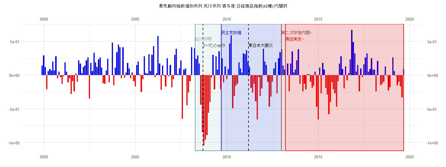
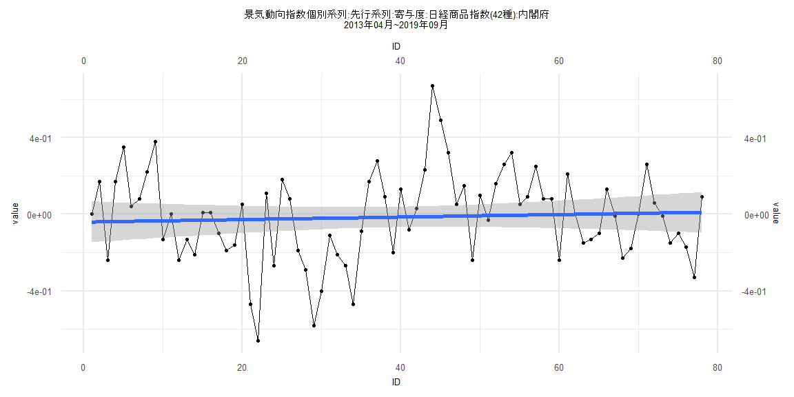
[1] "景気動向指数個別系列:先行系列:寄与度:日経商品指数(42種):内閣府"
       Jan   Feb   Mar   Apr   May   Jun   Jul   Aug   Sep   Oct   Nov   Dec
1999                                                                    0.14
2000  0.29  0.12 -0.21  0.06  0.09  0.07  0.20  0.07  0.28 -0.05  0.05 -0.03
2001 -0.13 -0.02  0.19  0.05 -0.11 -0.05 -0.28 -0.09 -0.24  0.02 -0.10  0.22
2002  0.17  0.03  0.12  0.14  0.22  0.26 -0.35  0.18  0.06  0.33  0.19  0.12
2003  0.23  0.26  0.11 -0.12 -0.13  0.07  0.24 -0.11  0.00  0.48 -0.15  0.11
2004  0.34  0.45  0.41 -0.05  0.41 -0.04  0.04  0.18  0.10 -0.05  0.04 -0.09
2005 -0.17  0.15  0.20  0.01 -0.25 -0.06  0.28  0.03  0.02  0.31  0.06  0.30
2006  0.43 -0.03  0.03  0.58  0.17 -0.22  0.14 -0.02 -0.17  0.25 -0.02  0.15
2007 -0.18 -0.06  0.30  0.39  0.01  0.10  0.22 -0.65  0.08  0.10 -0.45 -0.26
2008 -0.09  0.41  0.00  0.40  0.24  0.29  0.17 -0.44 -0.85 -1.04 -0.96 -0.89
2009 -0.56 -0.40 -0.04  0.30 -0.21  0.28  0.08  0.35 -0.21  0.25 -0.11  0.13
2010 -0.06  0.09  0.47  0.59 -0.49 -0.31 -0.16 -0.13  0.19  0.10  0.04  0.32
2011  0.31  0.37  0.20  0.12 -0.19 -0.26 -0.13 -0.39 -0.66 -0.03 -0.31 -0.20
2012  0.39  0.20  0.15 -0.10 -0.47 -0.32 -0.10  0.10  0.19 -0.27  0.25  0.34
2013  0.38  0.14  0.08  0.00  0.17 -0.24  0.17  0.35  0.04  0.08  0.22  0.38
2014 -0.13  0.00 -0.24 -0.13 -0.21  0.01  0.01 -0.10 -0.19 -0.16  0.05 -0.47
2015 -0.66  0.11 -0.27  0.18  0.08 -0.19 -0.29 -0.58 -0.40 -0.11 -0.21 -0.27
2016 -0.47 -0.09  0.17  0.28  0.09 -0.20  0.13 -0.08  0.03  0.23  0.67  0.49
2017  0.32  0.05  0.15 -0.24  0.10 -0.03  0.16  0.26  0.32  0.05  0.09  0.25
2018  0.08  0.08 -0.24  0.21  0.00 -0.15 -0.13 -0.10  0.13 -0.01 -0.23 -0.18
2019  0.00  0.26  0.06 -0.01 -0.15 -0.10 -0.17 -0.33  0.09
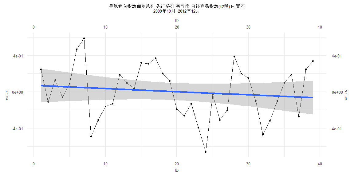
Call:
lm(formula = value ~ ID)

Residuals:
     Min       1Q   Median       3Q      Max
-0.64889 -0.19523  0.01629  0.20937  0.54192

Coefficients:
             Estimate Std. Error t value Pr(>|t|)
(Intercept)  0.072456   0.094945   0.763    0.450
ID          -0.003482   0.004137  -0.842    0.405

Residual standard error: 0.2908 on 37 degrees of freedom
Multiple R-squared:  0.01878,   Adjusted R-squared:  -0.007737
F-statistic: 0.7083 on 1 and 37 DF,  p-value: 0.4054


    Two-sample Kolmogorov-Smirnov test

data:  lm_residuals and rnorm(n = length(lm_residuals), mean = 0, sd = sd(lm_residuals))
D = 0.15385, p-value = 0.7523
alternative hypothesis: two-sided


    Durbin-Watson test

data:  value ~ ID
DW = 1.2148, p-value = 0.00292
alternative hypothesis: true autocorrelation is greater than 0


    studentized Breusch-Pagan test

data:  value ~ ID
BP = 0.0097755, df = 1, p-value = 0.9212


    Box-Ljung test

data:  lm_residuals
X-squared = 5.4954, df = 1, p-value = 0.01907
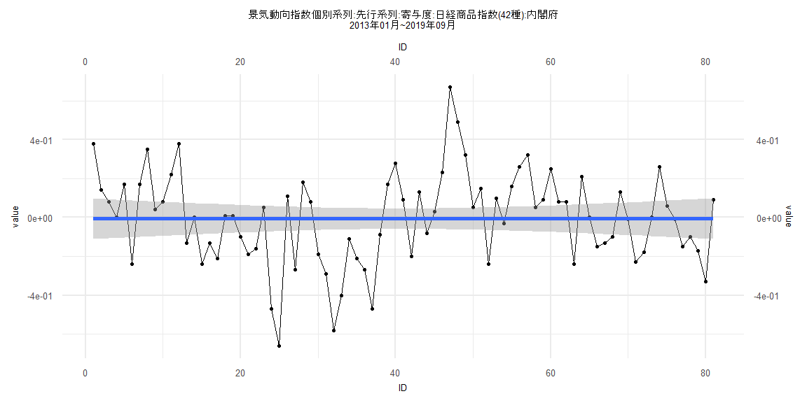
Call:
lm(formula = value ~ ID)

Residuals:
     Min       1Q   Median       3Q      Max
-0.65296 -0.16338  0.01708  0.14721  0.67687

Coefficients:
                Estimate   Std. Error t value Pr(>|t|)
(Intercept) -0.007228395  0.053366013  -0.135    0.893
ID           0.000007678  0.001130680   0.007    0.995

Residual standard error: 0.2379 on 79 degrees of freedom
Multiple R-squared:  5.838e-07, Adjusted R-squared:  -0.01266
F-statistic: 4.612e-05 on 1 and 79 DF,  p-value: 0.9946


    Two-sample Kolmogorov-Smirnov test

data:  lm_residuals and rnorm(n = length(lm_residuals), mean = 0, sd = sd(lm_residuals))
D = 0.17284, p-value = 0.1783
alternative hypothesis: two-sided


    Durbin-Watson test

data:  value ~ ID
DW = 1.0932, p-value = 0.000004238
alternative hypothesis: true autocorrelation is greater than 0


    studentized Breusch-Pagan test

data:  value ~ ID
BP = 1.0238, df = 1, p-value = 0.3116


    Box-Ljung test

data:  lm_residuals
X-squared = 15.947, df = 1, p-value = 0.00006513
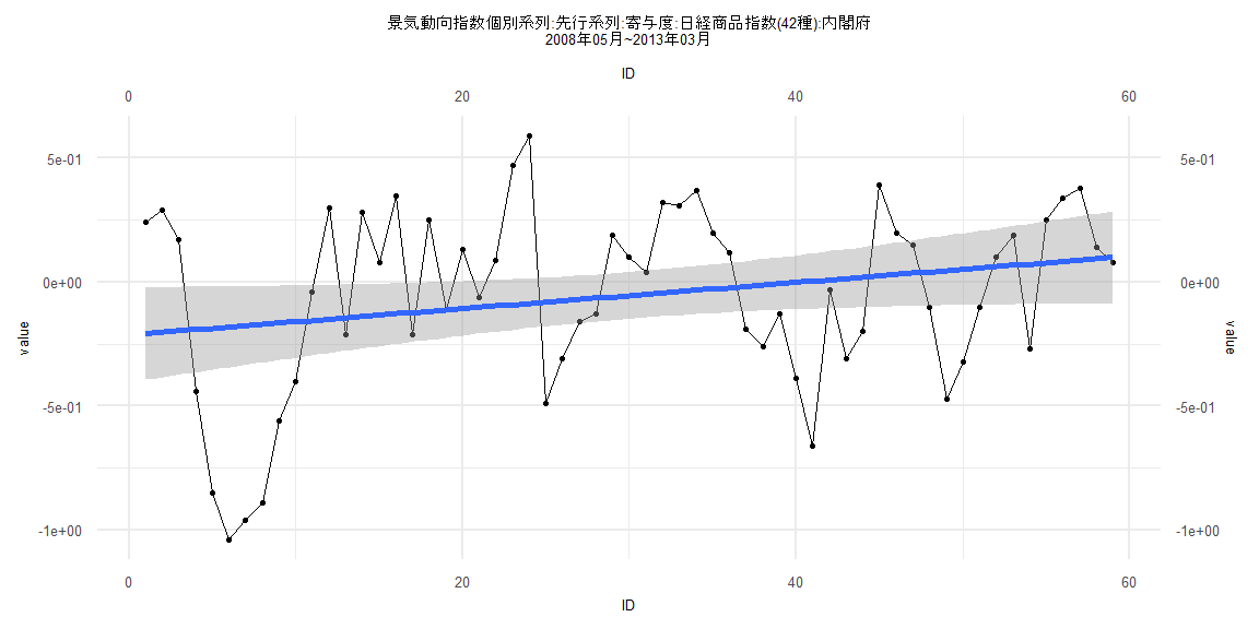
Call:
lm(formula = value ~ ID)

Residuals:
     Min       1Q   Median       3Q      Max
-0.85909 -0.23759  0.04153  0.25275  0.67565

Coefficients:
             Estimate Std. Error t value Pr(>|t|)
(Intercept) -0.212665   0.095351  -2.230   0.0297 *
ID           0.005292   0.002764   1.915   0.0606 .
---
Signif. codes:  0 '***' 0.001 '**' 0.01 '*' 0.05 '.' 0.1 ' ' 1

Residual standard error: 0.3616 on 57 degrees of freedom
Multiple R-squared:  0.06043,   Adjusted R-squared:  0.04394
F-statistic: 3.666 on 1 and 57 DF,  p-value: 0.06056


    Two-sample Kolmogorov-Smirnov test

data:  lm_residuals and rnorm(n = length(lm_residuals), mean = 0, sd = sd(lm_residuals))
D = 0.13559, p-value = 0.6544
alternative hypothesis: two-sided


    Durbin-Watson test

data:  value ~ ID
DW = 0.80362, p-value = 0.00000006211
alternative hypothesis: true autocorrelation is greater than 0


    studentized Breusch-Pagan test

data:  value ~ ID
BP = 9.7424, df = 1, p-value = 0.001801


    Box-Ljung test

data:  lm_residuals
X-squared = 21.216, df = 1, p-value = 0.000004102
Call:
lm(formula = value ~ ID)

Residuals:
     Min       1Q   Median       3Q      Max
-0.63372 -0.16551  0.03671  0.14232  0.68194

Coefficients:
             Estimate Std. Error t value Pr(>|t|)
(Intercept) -0.040626   0.054207  -0.749    0.456
ID           0.000652   0.001192   0.547    0.586

Residual standard error: 0.2371 on 76 degrees of freedom
Multiple R-squared:  0.00392,   Adjusted R-squared:  -0.009187
F-statistic: 0.2991 on 1 and 76 DF,  p-value: 0.5861


    Two-sample Kolmogorov-Smirnov test

data:  lm_residuals and rnorm(n = length(lm_residuals), mean = 0, sd = sd(lm_residuals))
D = 0.12821, p-value = 0.546
alternative hypothesis: two-sided


    Durbin-Watson test

data:  value ~ ID
DW = 1.1286, p-value = 0.00001402
alternative hypothesis: true autocorrelation is greater than 0


    studentized Breusch-Pagan test

data:  value ~ ID
BP = 1.0184, df = 1, p-value = 0.3129


    Box-Ljung test

data:  lm_residuals
X-squared = 15.317, df = 1, p-value = 0.0000909