Analysis
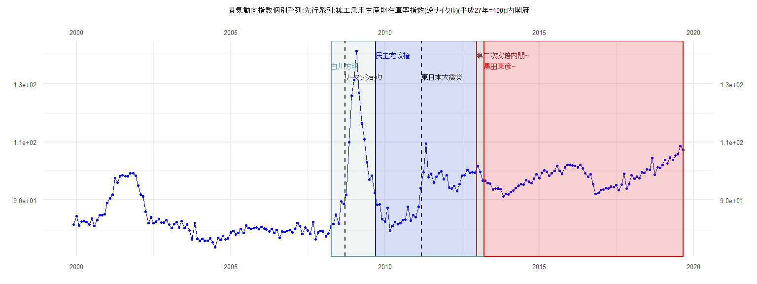
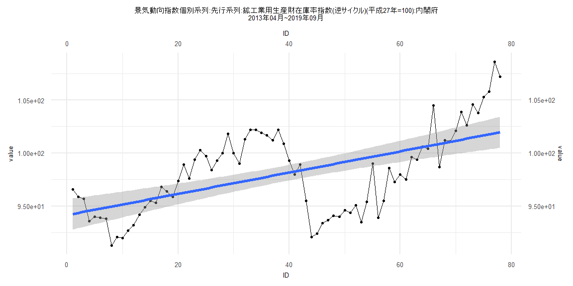
[1] "景気動向指数個別系列:先行系列:鉱工業用生産財在庫率指数(逆サイクル)(平成27年=100):内閣府"
       Jan   Feb   Mar   Apr   May   Jun   Jul   Aug   Sep   Oct   Nov   Dec
1999                                                                    81.5
2000  84.5  81.2  82.6  82.8  82.4  81.6  83.6  81.0  83.0  84.7  84.8  85.1
2001  89.0  90.5  91.7  97.6  96.0  98.2  98.6  98.2  98.2  99.2  99.2  98.4
2002  95.0  92.0  91.3  85.9  82.0  84.1  82.0  82.6  83.5  82.2  82.2  83.0
2003  81.5  80.3  81.8  82.4  80.5  82.8  80.4  81.5  79.5  76.5  82.1  76.7
2004  76.0  76.7  76.0  76.0  76.8  75.5  73.8  77.0  76.3  77.7  76.4  76.8
2005  78.8  79.3  78.1  78.7  80.0  78.7  81.2  80.4  80.1  80.3  80.5  80.1
2006  80.7  80.2  79.9  79.2  80.0  78.6  79.6  77.0  79.2  79.0  79.4  79.6
2007  78.8  80.0  82.0  81.0  78.3  80.5  79.5  78.3  82.4  76.5  78.8  79.3
2008  79.2  77.4  78.5  80.9  81.8  85.0  81.9  89.5  88.7  91.8 109.9 125.9
2009 131.4 141.4 126.9 116.4 111.0 103.0  97.0  98.4  92.4  88.3  88.5  83.5
2010  82.6  87.3  79.5  81.0  82.4  81.7  82.1  83.0  83.2  87.6  82.9  84.8
2011  84.1  87.6  94.2  99.5 109.5  97.8  99.0  96.0  98.0  99.3  99.9  97.2
2012  98.5  94.3  94.0  94.8  93.1  95.5  98.3  98.5 100.5  99.4  99.5  99.4
2013 101.7  99.8  96.7  96.6  95.9  95.7  93.6  94.0  93.9  93.8  91.3  92.1
2014  92.0  92.7  93.2  94.2  94.9  95.5  95.3  96.8  96.4  95.9  97.4  98.9
2015  97.6  99.4 100.3  99.7  98.4  99.3 100.0 101.8 100.0  99.0 101.3 102.2
2016 102.2 101.9 101.7 101.2 102.2 100.9  99.3  98.0  98.9  95.5  92.1  92.4
2017  93.4  93.7  94.1  94.0  94.6  94.4  95.1  93.5  95.4  99.0  93.9  95.5
2018  98.6  97.3  98.0  97.5  99.6  99.4 100.6 100.4 104.5  98.7 101.2 101.1
2019 102.1 103.9 102.6 104.6 103.8 105.3 105.8 108.6 107.2
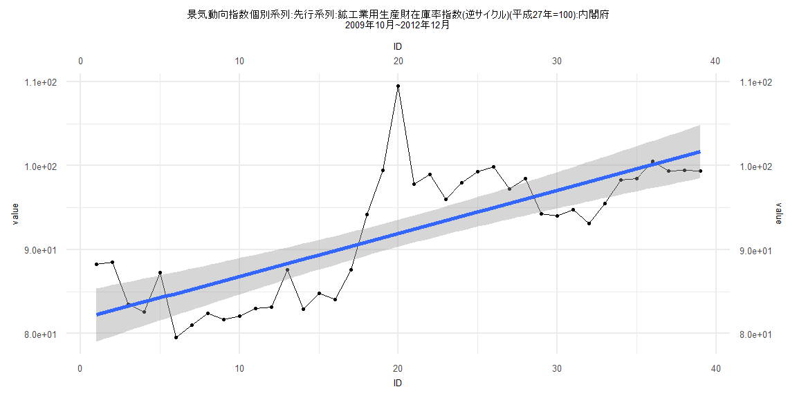
Call:
lm(formula = value ~ ID)

Residuals:
   Min     1Q Median     3Q    Max
-5.982 -3.851 -1.158  3.149 17.544

Coefficients:
            Estimate Std. Error t value             Pr(>|t|)
(Intercept) 81.70823    1.62529  50.273 < 0.0000000000000002 ***
ID           0.51241    0.07082   7.235         0.0000000138 ***
---
Signif. codes:  0 '***' 0.001 '**' 0.01 '*' 0.05 '.' 0.1 ' ' 1

Residual standard error: 4.978 on 37 degrees of freedom
Multiple R-squared:  0.5859,    Adjusted R-squared:  0.5747
F-statistic: 52.35 on 1 and 37 DF,  p-value: 0.0000000138


    Two-sample Kolmogorov-Smirnov test

data:  lm_residuals and rnorm(n = length(lm_residuals), mean = 0, sd = sd(lm_residuals))
D = 0.28205, p-value = 0.08974
alternative hypothesis: two-sided


    Durbin-Watson test

data:  value ~ ID
DW = 0.59452, p-value = 0.00000003294
alternative hypothesis: true autocorrelation is greater than 0


    studentized Breusch-Pagan test

data:  value ~ ID
BP = 0.43466, df = 1, p-value = 0.5097


    Box-Ljung test

data:  lm_residuals
X-squared = 19.441, df = 1, p-value = 0.00001038
Call:
lm(formula = value ~ ID)

Residuals:
    Min      1Q  Median      3Q     Max
-6.5756 -2.6352  0.2779  2.6536  7.0910

Coefficients:
            Estimate Std. Error t value             Pr(>|t|)
(Intercept) 94.64031    0.75880  124.72 < 0.0000000000000002 ***
ID           0.08586    0.01608    5.34          0.000000868 ***
---
Signif. codes:  0 '***' 0.001 '**' 0.01 '*' 0.05 '.' 0.1 ' ' 1

Residual standard error: 3.383 on 79 degrees of freedom
Multiple R-squared:  0.2653,    Adjusted R-squared:  0.256
F-statistic: 28.52 on 1 and 79 DF,  p-value: 0.000000868


    Two-sample Kolmogorov-Smirnov test

data:  lm_residuals and rnorm(n = length(lm_residuals), mean = 0, sd = sd(lm_residuals))
D = 0.11111, p-value = 0.7027
alternative hypothesis: two-sided


    Durbin-Watson test

data:  value ~ ID
DW = 0.26112, p-value < 0.00000000000000022
alternative hypothesis: true autocorrelation is greater than 0


    studentized Breusch-Pagan test

data:  value ~ ID
BP = 2.7001, df = 1, p-value = 0.1003


    Box-Ljung test

data:  lm_residuals
X-squared = 57.222, df = 1, p-value = 0.00000000000003897
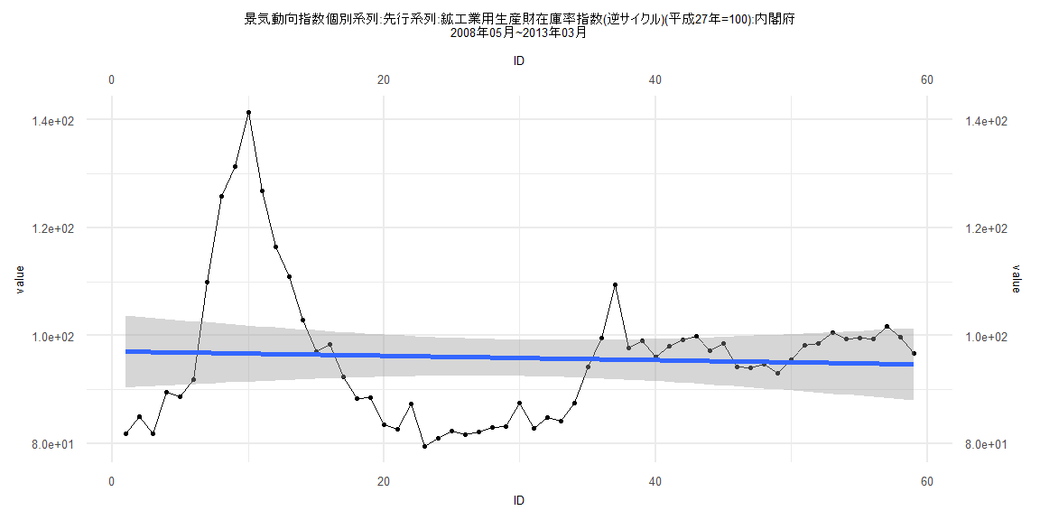
Call:
lm(formula = value ~ ID)

Residuals:
    Min      1Q  Median      3Q     Max
-16.662  -9.951   0.428   4.518  44.712

Coefficients:
            Estimate Std. Error t value            Pr(>|t|)
(Intercept) 97.09158    3.41735  28.411 <0.0000000000000002 ***
ID          -0.04040    0.09906  -0.408               0.685
---
Signif. codes:  0 '***' 0.001 '**' 0.01 '*' 0.05 '.' 0.1 ' ' 1

Residual standard error: 12.96 on 57 degrees of freedom
Multiple R-squared:  0.002909,  Adjusted R-squared:  -0.01458
F-statistic: 0.1663 on 1 and 57 DF,  p-value: 0.685


    Two-sample Kolmogorov-Smirnov test

data:  lm_residuals and rnorm(n = length(lm_residuals), mean = 0, sd = sd(lm_residuals))
D = 0.30508, p-value = 0.00792
alternative hypothesis: two-sided


    Durbin-Watson test

data:  value ~ ID
DW = 0.19563, p-value < 0.00000000000000022
alternative hypothesis: true autocorrelation is greater than 0


    studentized Breusch-Pagan test

data:  value ~ ID
BP = 10.811, df = 1, p-value = 0.001009


    Box-Ljung test

data:  lm_residuals
X-squared = 49.132, df = 1, p-value = 0.000000000002393
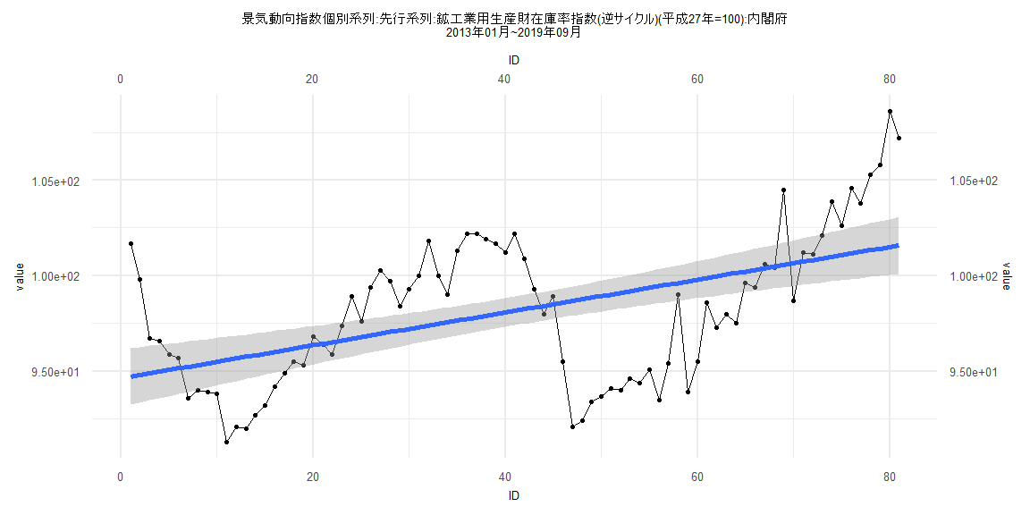
Call:
lm(formula = value ~ ID)

Residuals:
    Min      1Q  Median      3Q     Max
-6.4632 -2.4616  0.0348  2.7876  6.7339

Coefficients:
            Estimate Std. Error t value             Pr(>|t|)
(Intercept) 94.15937    0.74966  125.60 < 0.0000000000000002 ***
ID           0.10009    0.01649    6.07         0.0000000466 ***
---
Signif. codes:  0 '***' 0.001 '**' 0.01 '*' 0.05 '.' 0.1 ' ' 1

Residual standard error: 3.279 on 76 degrees of freedom
Multiple R-squared:  0.3265,    Adjusted R-squared:  0.3177
F-statistic: 36.85 on 1 and 76 DF,  p-value: 0.00000004663


    Two-sample Kolmogorov-Smirnov test

data:  lm_residuals and rnorm(n = length(lm_residuals), mean = 0, sd = sd(lm_residuals))
D = 0.12821, p-value = 0.546
alternative hypothesis: two-sided


    Durbin-Watson test

data:  value ~ ID
DW = 0.27158, p-value < 0.00000000000000022
alternative hypothesis: true autocorrelation is greater than 0


    studentized Breusch-Pagan test

data:  value ~ ID
BP = 6.3501, df = 1, p-value = 0.01174


    Box-Ljung test

data:  lm_residuals
X-squared = 57.74, df = 1, p-value = 0.00000000000002998