Analysis
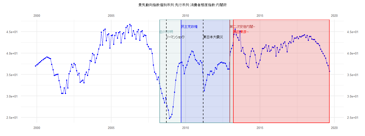
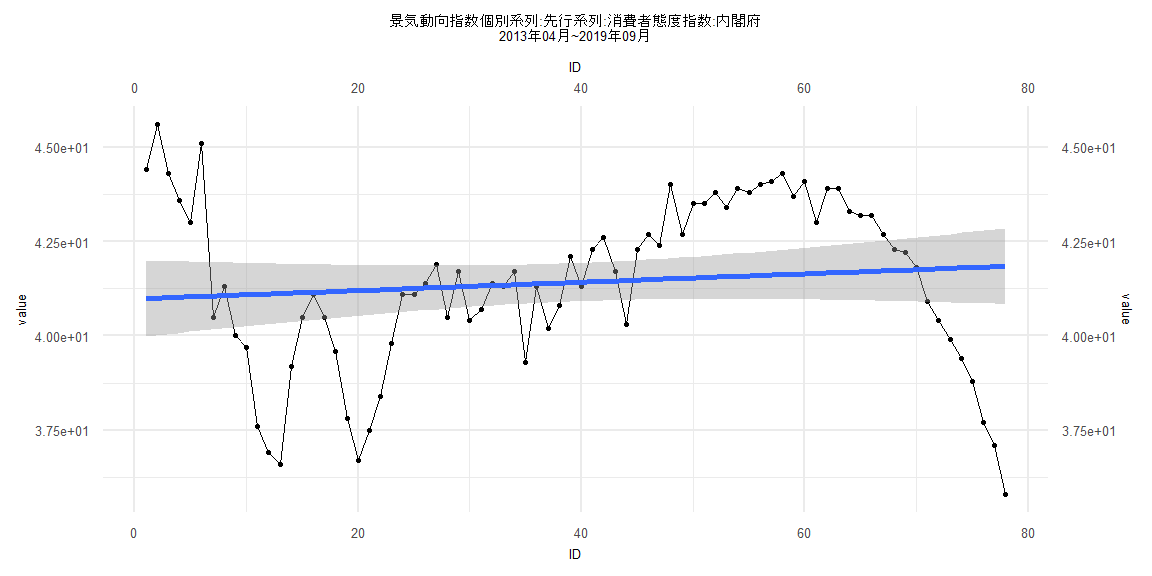
[1] "景気動向指数個別系列:先行系列:消費者態度指数:内閣府"
      Jan  Feb  Mar  Apr  May  Jun  Jul  Aug  Sep  Oct  Nov  Dec
1999                                                        37.0
2000 37.3 37.5 37.8 38.0 38.3 38.5 38.7 38.9 39.1 39.0 38.8 38.7
2001 37.4 36.1 34.8 34.9 35.0 35.1 33.6 32.1 30.6 30.6 31.9 30.6
2002 33.7 31.9 35.2 35.8 37.4 36.7 37.6 37.3 35.9 34.9 35.3 33.2
2003 33.5 33.7 33.1 35.0 35.6 34.8 36.2 38.3 38.1 39.9 39.6 37.8
2004 38.8 39.7 41.0 41.9 44.9 41.9 45.3 45.6 42.9 44.3 44.5 41.2
2005 44.1 44.2 42.1 44.1 44.8 43.5 44.8 45.0 42.4 44.5 44.8 43.4
2006 46.0 46.4 44.8 46.7 46.4 44.0 45.2 44.4 43.3 45.0 45.5 43.0
2007 45.0 45.2 43.9 44.2 44.1 42.0 41.5 41.0 41.0 39.9 37.2 35.6
2008 35.2 33.8 34.4 32.9 31.7 30.6 29.4 28.4 29.6 27.7 26.7 24.8
2009 25.1 25.7 27.5 30.9 33.7 35.4 36.9 37.6 37.8 37.9 37.1 35.2
2010 36.6 37.2 38.1 39.1 39.7 40.5 40.3 39.5 38.5 38.2 37.7 37.4
2011 38.2 37.8 35.6 31.2 32.6 33.7 35.0 34.9 35.8 35.8 35.0 35.4
2012 36.6 36.3 37.3 37.5 37.8 37.9 37.7 37.7 37.6 37.0 36.3 36.3
2013 40.3 41.1 41.8 44.4 45.6 44.3 43.6 43.0 45.1 40.5 41.3 40.0
2014 39.7 37.6 36.9 36.6 39.2 40.5 41.1 40.5 39.6 37.8 36.7 37.5
2015 38.4 39.8 41.1 41.1 41.4 41.9 40.5 41.7 40.4 40.7 41.4 41.3
2016 41.7 39.3 41.3 40.2 40.8 42.1 41.3 42.3 42.6 41.7 40.3 42.3
2017 42.7 42.4 44.0 42.7 43.5 43.5 43.8 43.4 43.9 43.8 44.0 44.1
2018 44.3 43.7 44.1 43.0 43.9 43.9 43.3 43.2 43.2 42.7 42.3 42.2
2019 41.8 40.9 40.4 39.9 39.4 38.8 37.7 37.1 35.8
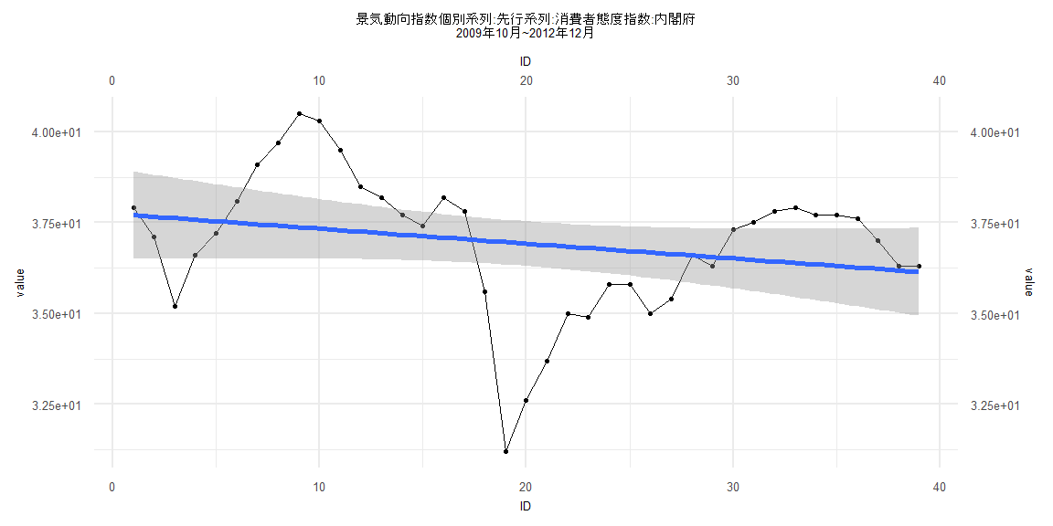
Call:
lm(formula = value ~ ID)

Residuals:
   Min     1Q Median     3Q    Max
-5.764 -0.969  0.272  1.291  3.126

Coefficients:
            Estimate Std. Error t value            Pr(>|t|)
(Intercept) 37.74291    0.61884   60.99 <0.0000000000000002 ***
ID          -0.04099    0.02697   -1.52               0.137
---
Signif. codes:  0 '***' 0.001 '**' 0.01 '*' 0.05 '.' 0.1 ' ' 1

Residual standard error: 1.895 on 37 degrees of freedom
Multiple R-squared:  0.05878,   Adjusted R-squared:  0.03335
F-statistic: 2.311 on 1 and 37 DF,  p-value: 0.137


    Two-sample Kolmogorov-Smirnov test

data:  lm_residuals and rnorm(n = length(lm_residuals), mean = 0, sd = sd(lm_residuals))
D = 0.20513, p-value = 0.3888
alternative hypothesis: two-sided


    Durbin-Watson test

data:  value ~ ID
DW = 0.34966, p-value = 0.00000000000158
alternative hypothesis: true autocorrelation is greater than 0


    studentized Breusch-Pagan test

data:  value ~ ID
BP = 0.50449, df = 1, p-value = 0.4775


    Box-Ljung test

data:  lm_residuals
X-squared = 28.635, df = 1, p-value = 0.00000008738
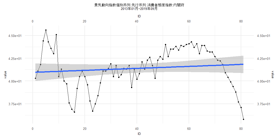
Call:
lm(formula = value ~ ID)

Residuals:
    Min      1Q  Median      3Q     Max
-6.0379 -1.1688  0.1266  1.6140  4.5871

Coefficients:
            Estimate Std. Error t value            Pr(>|t|)
(Intercept) 40.95861    0.49477  82.783 <0.0000000000000002 ***
ID           0.01086    0.01048   1.036               0.304
---
Signif. codes:  0 '***' 0.001 '**' 0.01 '*' 0.05 '.' 0.1 ' ' 1

Residual standard error: 2.206 on 79 degrees of freedom
Multiple R-squared:  0.01339,   Adjusted R-squared:  0.0009047
F-statistic: 1.072 on 1 and 79 DF,  p-value: 0.3036


    Two-sample Kolmogorov-Smirnov test

data:  lm_residuals and rnorm(n = length(lm_residuals), mean = 0, sd = sd(lm_residuals))
D = 0.14815, p-value = 0.338
alternative hypothesis: two-sided


    Durbin-Watson test

data:  value ~ ID
DW = 0.2773, p-value < 0.00000000000000022
alternative hypothesis: true autocorrelation is greater than 0


    studentized Breusch-Pagan test

data:  value ~ ID
BP = 0.038484, df = 1, p-value = 0.8445


    Box-Ljung test

data:  lm_residuals
X-squared = 55.594, df = 1, p-value = 0.00000000000008915
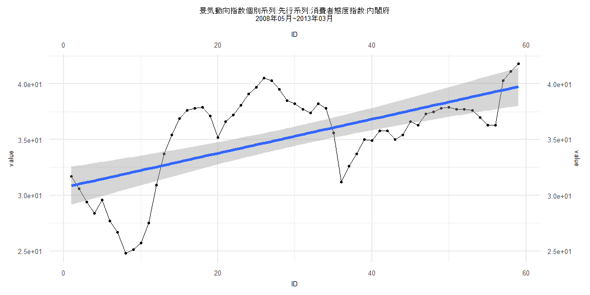
Call:
lm(formula = value ~ ID)

Residuals:
    Min      1Q  Median      3Q     Max
-7.1243 -1.9585 -0.4688  2.6180  5.8138

Coefficients:
            Estimate Std. Error t value             Pr(>|t|)
(Intercept) 30.69673    0.87467  35.095 < 0.0000000000000002 ***
ID           0.15344    0.02536   6.052          0.000000118 ***
---
Signif. codes:  0 '***' 0.001 '**' 0.01 '*' 0.05 '.' 0.1 ' ' 1

Residual standard error: 3.317 on 57 degrees of freedom
Multiple R-squared:  0.3912,    Adjusted R-squared:  0.3805
F-statistic: 36.62 on 1 and 57 DF,  p-value: 0.0000001183


    Two-sample Kolmogorov-Smirnov test

data:  lm_residuals and rnorm(n = length(lm_residuals), mean = 0, sd = sd(lm_residuals))
D = 0.084746, p-value = 0.9854
alternative hypothesis: two-sided


    Durbin-Watson test

data:  value ~ ID
DW = 0.1659, p-value < 0.00000000000000022
alternative hypothesis: true autocorrelation is greater than 0


    studentized Breusch-Pagan test

data:  value ~ ID
BP = 11.837, df = 1, p-value = 0.0005807


    Box-Ljung test

data:  lm_residuals
X-squared = 51.738, df = 1, p-value = 0.000000000000634
Call:
lm(formula = value ~ ID)

Residuals:
    Min      1Q  Median      3Q     Max
-6.0434 -1.1834  0.1827  1.7782  4.5990

Coefficients:
            Estimate Std. Error t value            Pr(>|t|)
(Intercept) 40.97885    0.51349  79.805 <0.0000000000000002 ***
ID           0.01108    0.01129   0.981                0.33
---
Signif. codes:  0 '***' 0.001 '**' 0.01 '*' 0.05 '.' 0.1 ' ' 1

Residual standard error: 2.246 on 76 degrees of freedom
Multiple R-squared:  0.01251,   Adjusted R-squared:  -0.0004787
F-statistic: 0.9632 on 1 and 76 DF,  p-value: 0.3295


    Two-sample Kolmogorov-Smirnov test

data:  lm_residuals and rnorm(n = length(lm_residuals), mean = 0, sd = sd(lm_residuals))
D = 0.15385, p-value = 0.316
alternative hypothesis: two-sided


    Durbin-Watson test

data:  value ~ ID
DW = 0.25777, p-value < 0.00000000000000022
alternative hypothesis: true autocorrelation is greater than 0


    studentized Breusch-Pagan test

data:  value ~ ID
BP = 0.034965, df = 1, p-value = 0.8517


    Box-Ljung test

data:  lm_residuals
X-squared = 52.947, df = 1, p-value = 0.0000000000003426