Analysis
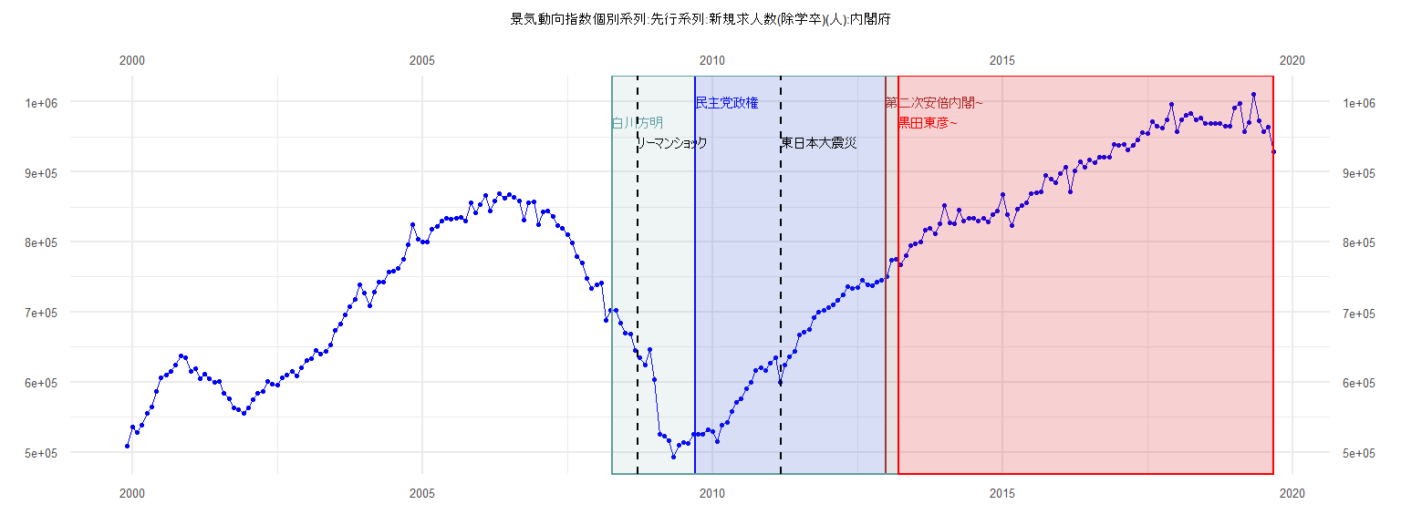
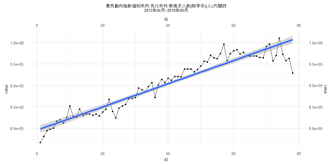
[1] "景気動向指数個別系列:先行系列:新規求人数(除学卒)(人):内閣府"
         Jan     Feb     Mar     Apr     May     Jun     Jul     Aug     Sep     Oct     Nov     Dec
1999                                                                                          508316
2000  535617  528372  538001  555144  564639  585988  605865  610257  615264  624621  637409  634688
2001  615461  618640  604612  611569  604371  599274  601079  583771  576815  562524  560059  555381
2002  562867  574291  584478  587126  600442  597383  595328  606017  610380  615006  608816  619766
2003  631081  633411  645082  640289  644419  653360  674017  682251  696374  707533  718043  739086
2004  727646  708340  728859  742912  742782  756655  758830  762017  775746  796232  824611  803400
2005  800057  800017  818414  821530  829649  834263  832003  834107  834544  829994  855905  841041
2006  852862  865769  844771  858312  869166  861830  867435  863916  857953  830677  855417  856829
2007  825291  842244  844035  836212  823085  819578  810943  799197  779312  769743  748010  733423
2008  738734  741011  687760  702162  702404  684611  670503  669081  645485  634327  623862  646836
2009  603284  525404  523109  516148  493498  509473  513653  512577  525120  524960  525780  532497
2010  529683  515424  537858  542156  557609  571488  575767  590956  599830  616858  619941  616063
2011  627421  635217  599542  623808  635577  643256  667304  671104  675209  692019  700299  702410
2012  706425  710037  716249  724667  735556  733296  734553  744934  738931  737931  742311  745455
2013  750781  774550  775531  766816  780614  794192  797506  800444  816314  819874  811925  825575
2014  852362  827686  825784  844984  829644  833406  833746  829938  833538  828575  838352  844312
2015  868013  839582  823788  847212  852504  855864  869209  870118  871639  894332  890336  884997
2016  897626  907127  872140  901378  914532  906562  917058  912568  920949  920906  920400  938650
2017  938304  938848  931597  937423  945346  956523  954503  971134  964972  962865  973921  996450
2018  957306  974537  981150  983720  973666  977335  969651  968758  968853  969084  965689  964901
2019  990914  997446  957235  969912 1010637  973112  957810  963439  928972
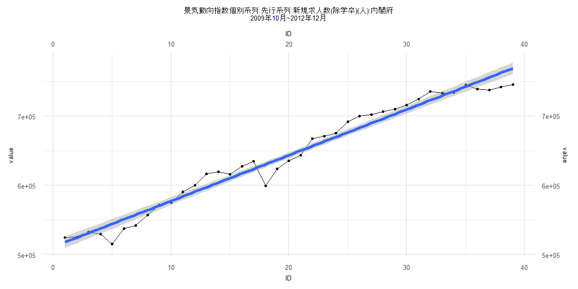
Call:
lm(formula = value ~ ID)

Residuals:
   Min     1Q Median     3Q    Max
-30830  -8058   3716   9528  19556

Coefficients:
            Estimate Std. Error t value            Pr(>|t|)
(Intercept) 511321.3     4302.1  118.85 <0.0000000000000002 ***
ID            6613.9      187.5   35.28 <0.0000000000000002 ***
---
Signif. codes:  0 '***' 0.001 '**' 0.01 '*' 0.05 '.' 0.1 ' ' 1

Residual standard error: 13180 on 37 degrees of freedom
Multiple R-squared:  0.9711,    Adjusted R-squared:  0.9704
F-statistic:  1245 on 1 and 37 DF,  p-value: < 0.00000000000000022


    Two-sample Kolmogorov-Smirnov test

data:  lm_residuals and rnorm(n = length(lm_residuals), mean = 0, sd = sd(lm_residuals))
D = 0.25641, p-value = 0.1547
alternative hypothesis: two-sided


    Durbin-Watson test

data:  value ~ ID
DW = 0.66164, p-value = 0.0000002169
alternative hypothesis: true autocorrelation is greater than 0


    studentized Breusch-Pagan test

data:  value ~ ID
BP = 0.14126, df = 1, p-value = 0.707


    Box-Ljung test

data:  lm_residuals
X-squared = 16.239, df = 1, p-value = 0.00005584
Call:
lm(formula = value ~ ID)

Residuals:
   Min     1Q Median     3Q    Max
-79925  -9313   4031  13842  45956

Coefficients:
             Estimate Std. Error t value            Pr(>|t|)
(Intercept) 783629.83    4485.86  174.69 <0.0000000000000002 ***
ID            2781.07      95.04   29.26 <0.0000000000000002 ***
---
Signif. codes:  0 '***' 0.001 '**' 0.01 '*' 0.05 '.' 0.1 ' ' 1

Residual standard error: 20000 on 79 degrees of freedom
Multiple R-squared:  0.9155,    Adjusted R-squared:  0.9145
F-statistic: 856.2 on 1 and 79 DF,  p-value: < 0.00000000000000022


    Two-sample Kolmogorov-Smirnov test

data:  lm_residuals and rnorm(n = length(lm_residuals), mean = 0, sd = sd(lm_residuals))
D = 0.098765, p-value = 0.8277
alternative hypothesis: two-sided


    Durbin-Watson test

data:  value ~ ID
DW = 0.62241, p-value = 0.00000000000008349
alternative hypothesis: true autocorrelation is greater than 0


    studentized Breusch-Pagan test

data:  value ~ ID
BP = 7.6041, df = 1, p-value = 0.005824


    Box-Ljung test

data:  lm_residuals
X-squared = 27.077, df = 1, p-value = 0.0000001955
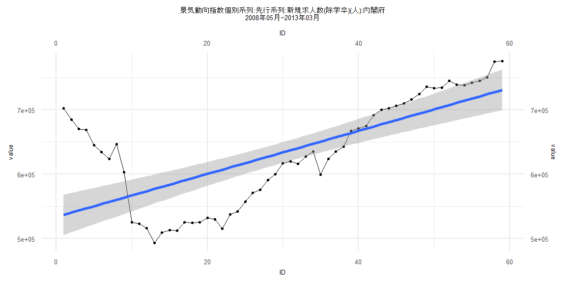
Call:
lm(formula = value ~ ID)

Residuals:
   Min     1Q Median     3Q    Max
-91745 -50065   3313  30522 165428

Coefficients:
            Estimate Std. Error t value             Pr(>|t|)
(Intercept) 533633.5    16152.7  33.037 < 0.0000000000000002 ***
ID            3342.5      468.2   7.138        0.00000000187 ***
---
Signif. codes:  0 '***' 0.001 '**' 0.01 '*' 0.05 '.' 0.1 ' ' 1

Residual standard error: 61250 on 57 degrees of freedom
Multiple R-squared:  0.472, Adjusted R-squared:  0.4627
F-statistic: 50.96 on 1 and 57 DF,  p-value: 0.000000001871


    Two-sample Kolmogorov-Smirnov test

data:  lm_residuals and rnorm(n = length(lm_residuals), mean = 0, sd = sd(lm_residuals))
D = 0.16949, p-value = 0.3674
alternative hypothesis: two-sided


    Durbin-Watson test

data:  value ~ ID
DW = 0.079754, p-value < 0.00000000000000022
alternative hypothesis: true autocorrelation is greater than 0


    studentized Breusch-Pagan test

data:  value ~ ID
BP = 26.179, df = 1, p-value = 0.0000003112


    Box-Ljung test

data:  lm_residuals
X-squared = 49.313, df = 1, p-value = 0.000000000002182
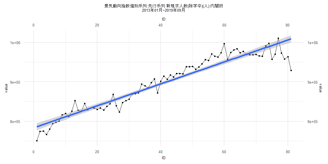
Call:
lm(formula = value ~ ID)

Residuals:
   Min     1Q Median     3Q    Max
-78130 -10495   4471  13889  46305

Coefficients:
             Estimate Std. Error t value            Pr(>|t|)
(Intercept) 795546.73    4512.48  176.30 <0.0000000000000002 ***
ID            2712.25      99.25   27.33 <0.0000000000000002 ***
---
Signif. codes:  0 '***' 0.001 '**' 0.01 '*' 0.05 '.' 0.1 ' ' 1

Residual standard error: 19740 on 76 degrees of freedom
Multiple R-squared:  0.9076,    Adjusted R-squared:  0.9064
F-statistic: 746.8 on 1 and 76 DF,  p-value: < 0.00000000000000022


    Two-sample Kolmogorov-Smirnov test

data:  lm_residuals and rnorm(n = length(lm_residuals), mean = 0, sd = sd(lm_residuals))
D = 0.11538, p-value = 0.6802
alternative hypothesis: two-sided


    Durbin-Watson test

data:  value ~ ID
DW = 0.64475, p-value = 0.000000000000717
alternative hypothesis: true autocorrelation is greater than 0


    studentized Breusch-Pagan test

data:  value ~ ID
BP = 8.2961, df = 1, p-value = 0.003973


    Box-Ljung test

data:  lm_residuals
X-squared = 25.216, df = 1, p-value = 0.0000005127