Analysis
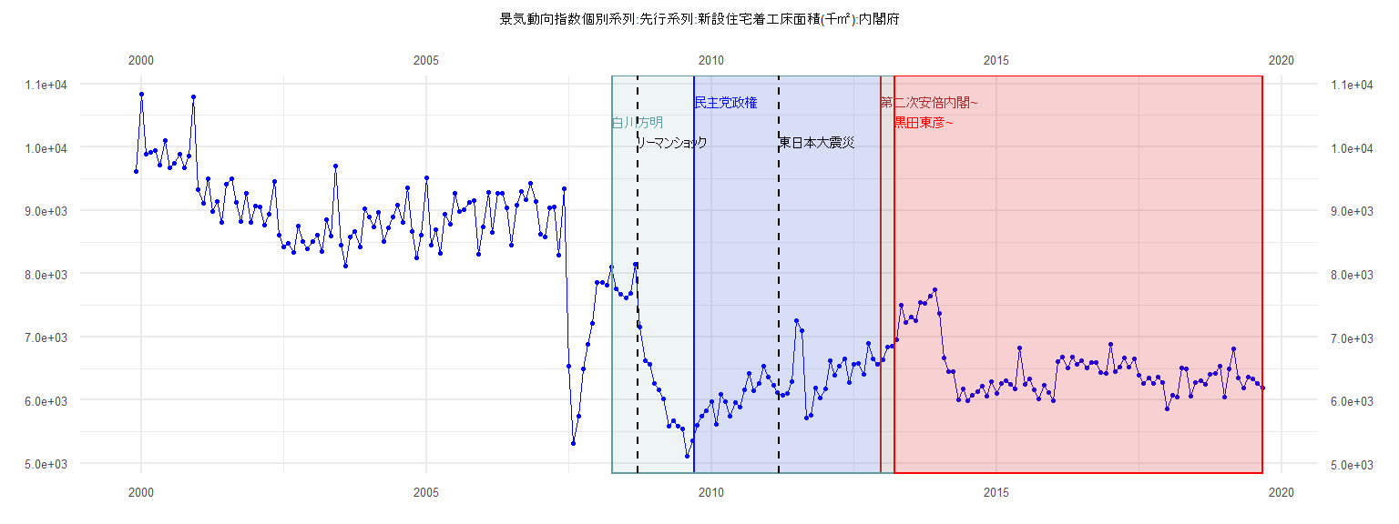
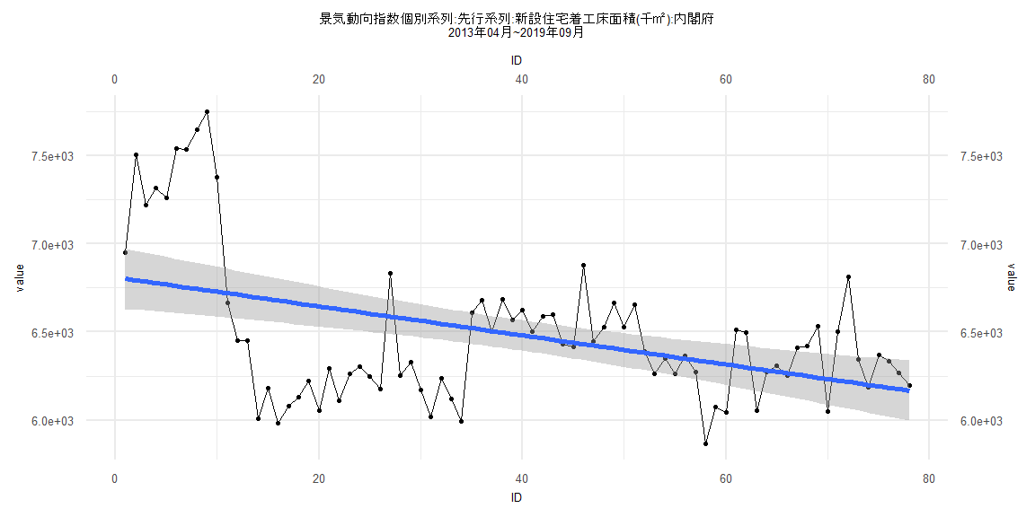
[1] "景気動向指数個別系列:先行系列:新設住宅着工床面積(千㎡):内閣府"
       Jan   Feb   Mar   Apr   May   Jun   Jul   Aug   Sep   Oct   Nov   Dec
1999                                                                    9615
2000 10837  9887  9924  9951  9721 10110  9674  9744  9894  9668  9864 10792
2001  9326  9115  9495  8988  9144  8817  9409  9498  9133  8824  9274  8806
2002  9070  9049  8762  8938  9464  8613  8425  8479  8342  8746  8512  8388
2003  8508  8609  8349  8850  8599  9698  8450  8114  8577  8663  8428  9025
2004  8897  8734  8961  8506  8728  8894  9084  8809  9362  8663  8249  8608
2005  9516  8451  8697  8325  8934  8780  9276  8979  9014  9133  9153  8302
2006  8734  9287  8650  9276  9273  9037  8452  9083  9295  9172  9425  9144
2007  8630  8585  9041  9050  8287  9345  6531  5313  5748  6494  6888  7213
2008  7857  7857  7813  8106  7758  7671  7619  7693  8142  7149  6628  6564
2009  6268  6161  6016  5585  5672  5584  5548  5120  5357  5605  5749  5834
2010  5977  5614  6090  5972  5746  5962  5889  6166  6419  6145  6263  6543
2011  6359  6233  6122  6073  6105  6300  7254  7102  5715  5758  6186  6036
2012  6184  6629  6389  6542  6654  6282  6569  6586  6406  6898  6652  6565
2013  6644  6836  6860  6950  7502  7222  7316  7261  7540  7535  7645  7748
2014  7376  6667  6450  6450  6008  6182  5984  6081  6133  6222  6057  6293
2015  6113  6264  6306  6248  6178  6832  6254  6330  6170  6021  6238  6123
2016  5994  6611  6680  6502  6684  6569  6622  6502  6590  6599  6432  6418
2017  6879  6446  6528  6666  6527  6653  6388  6261  6348  6263  6367  6274
2018  5867  6076  6044  6511  6495  6056  6276  6310  6255  6413  6422  6533
2019  6048  6500  6811  6345  6186  6368  6333  6268  6196
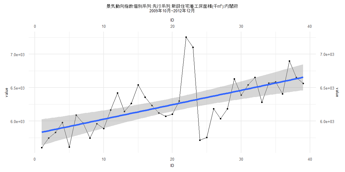
Call:
lm(formula = value ~ ID)

Residuals:
    Min      1Q  Median      3Q     Max
-616.86 -167.95    7.32  130.92  965.34

Coefficients:
            Estimate Std. Error t value             Pr(>|t|)
(Intercept) 5813.490     99.685  58.319 < 0.0000000000000002 ***
ID            21.599      4.344   4.972            0.0000154 ***
---
Signif. codes:  0 '***' 0.001 '**' 0.01 '*' 0.05 '.' 0.1 ' ' 1

Residual standard error: 305.3 on 37 degrees of freedom
Multiple R-squared:  0.4006,    Adjusted R-squared:  0.3844
F-statistic: 24.72 on 1 and 37 DF,  p-value: 0.00001536


    Two-sample Kolmogorov-Smirnov test

data:  lm_residuals and rnorm(n = length(lm_residuals), mean = 0, sd = sd(lm_residuals))
D = 0.12821, p-value = 0.9114
alternative hypothesis: two-sided


    Durbin-Watson test

data:  value ~ ID
DW = 1.4073, p-value = 0.01848
alternative hypothesis: true autocorrelation is greater than 0


    studentized Breusch-Pagan test

data:  value ~ ID
BP = 0.21036, df = 1, p-value = 0.6465


    Box-Ljung test

data:  lm_residuals
X-squared = 3.4779, df = 1, p-value = 0.06219
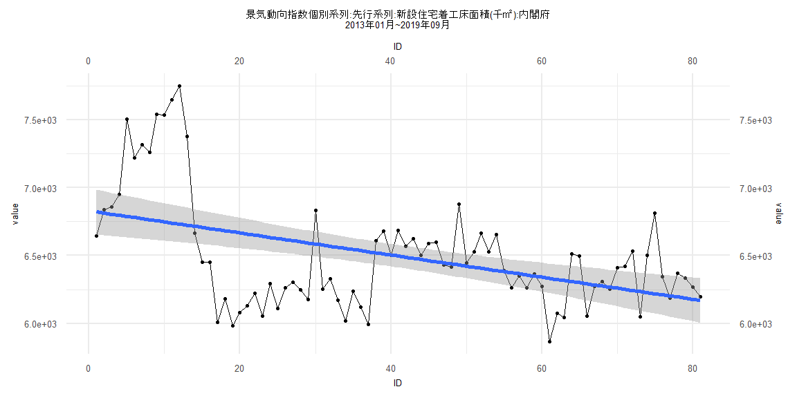
Call:
lm(formula = value ~ ID)

Residuals:
    Min      1Q  Median      3Q     Max
-690.66 -272.82   17.65  170.24 1016.41

Coefficients:
            Estimate Std. Error t value             Pr(>|t|)
(Intercept) 6829.179     84.018  81.283 < 0.0000000000000002 ***
ID            -8.133      1.780  -4.569            0.0000178 ***
---
Signif. codes:  0 '***' 0.001 '**' 0.01 '*' 0.05 '.' 0.1 ' ' 1

Residual standard error: 374.6 on 79 degrees of freedom
Multiple R-squared:  0.209, Adjusted R-squared:  0.199
F-statistic: 20.87 on 1 and 79 DF,  p-value: 0.00001784


    Two-sample Kolmogorov-Smirnov test

data:  lm_residuals and rnorm(n = length(lm_residuals), mean = 0, sd = sd(lm_residuals))
D = 0.08642, p-value = 0.9254
alternative hypothesis: two-sided


    Durbin-Watson test

data:  value ~ ID
DW = 0.46772, p-value < 0.00000000000000022
alternative hypothesis: true autocorrelation is greater than 0


    studentized Breusch-Pagan test

data:  value ~ ID
BP = 20.687, df = 1, p-value = 0.000005409


    Box-Ljung test

data:  lm_residuals
X-squared = 49.142, df = 1, p-value = 0.000000000002381
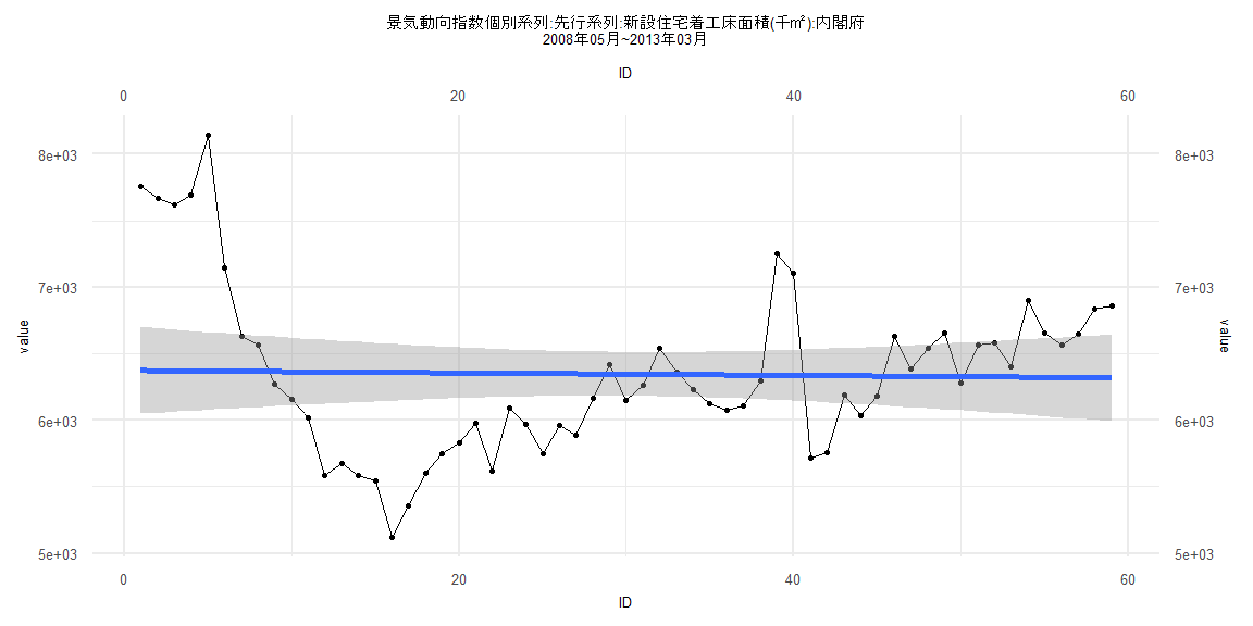
Call:
lm(formula = value ~ ID)

Residuals:
     Min       1Q   Median       3Q      Max
-1239.69  -384.26   -98.25   278.72  1772.01

Coefficients:
             Estimate Std. Error t value            Pr(>|t|)
(Intercept) 6374.6756   166.7512  38.229 <0.0000000000000002 ***
ID            -0.9366     4.8339  -0.194               0.847
---
Signif. codes:  0 '***' 0.001 '**' 0.01 '*' 0.05 '.' 0.1 ' ' 1

Residual standard error: 632.3 on 57 degrees of freedom
Multiple R-squared:  0.0006583, Adjusted R-squared:  -0.01687
F-statistic: 0.03755 on 1 and 57 DF,  p-value: 0.847


    Two-sample Kolmogorov-Smirnov test

data:  lm_residuals and rnorm(n = length(lm_residuals), mean = 0, sd = sd(lm_residuals))
D = 0.13559, p-value = 0.6544
alternative hypothesis: two-sided


    Durbin-Watson test

data:  value ~ ID
DW = 0.30811, p-value < 0.00000000000000022
alternative hypothesis: true autocorrelation is greater than 0


    studentized Breusch-Pagan test

data:  value ~ ID
BP = 17.206, df = 1, p-value = 0.00003354


    Box-Ljung test

data:  lm_residuals
X-squared = 39.465, df = 1, p-value = 0.0000000003341
Call:
lm(formula = value ~ ID)

Residuals:
    Min      1Q  Median      3Q     Max
-694.44 -297.87   12.17  174.78 1011.88

Coefficients:
            Estimate Std. Error t value             Pr(>|t|)
(Intercept) 6810.274     87.183  78.115 < 0.0000000000000002 ***
ID            -8.240      1.918  -4.297            0.0000507 ***
---
Signif. codes:  0 '***' 0.001 '**' 0.01 '*' 0.05 '.' 0.1 ' ' 1

Residual standard error: 381.3 on 76 degrees of freedom
Multiple R-squared:  0.1955,    Adjusted R-squared:  0.1849
F-statistic: 18.46 on 1 and 76 DF,  p-value: 0.00005068


    Two-sample Kolmogorov-Smirnov test

data:  lm_residuals and rnorm(n = length(lm_residuals), mean = 0, sd = sd(lm_residuals))
D = 0.15385, p-value = 0.316
alternative hypothesis: two-sided


    Durbin-Watson test

data:  value ~ ID
DW = 0.46463, p-value < 0.00000000000000022
alternative hypothesis: true autocorrelation is greater than 0


    studentized Breusch-Pagan test

data:  value ~ ID
BP = 26.501, df = 1, p-value = 0.0000002634


    Box-Ljung test

data:  lm_residuals
X-squared = 47.632, df = 1, p-value = 0.000000000005143