Analysis
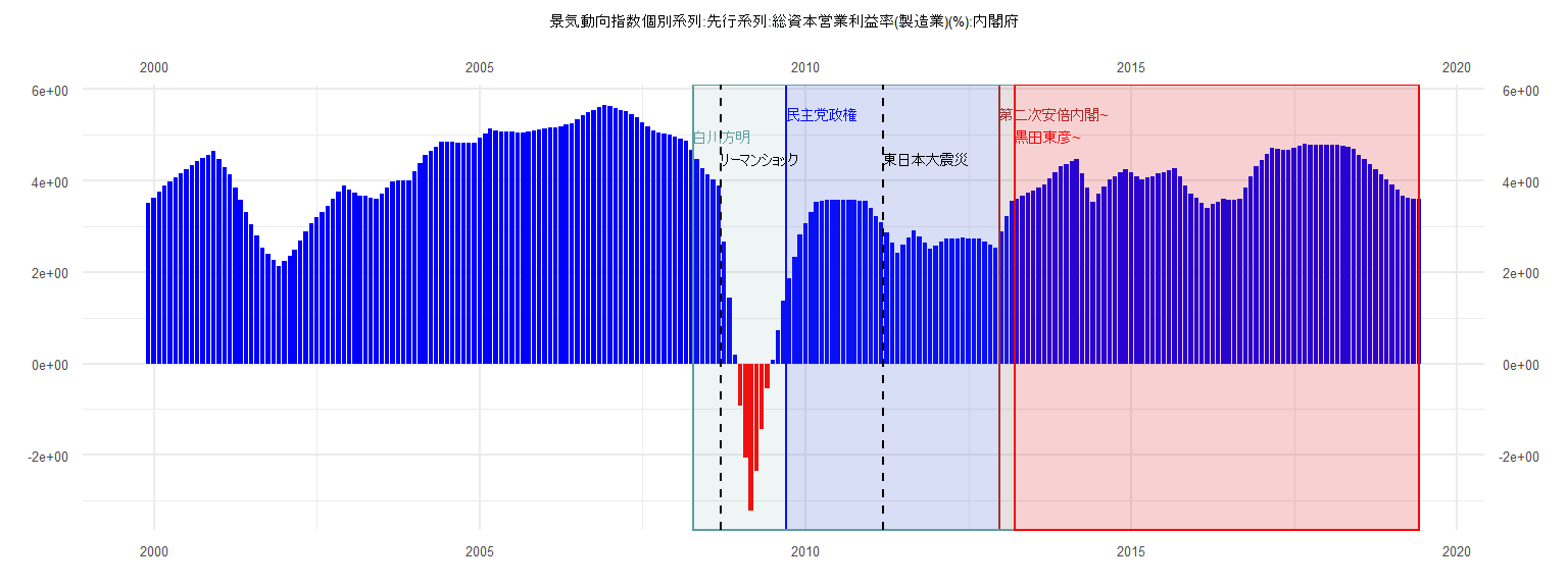
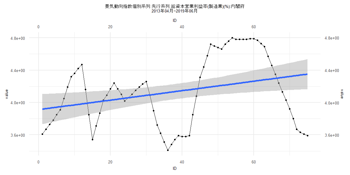
[1] "景気動向指数個別系列:先行系列:総資本営業利益率(製造業)(%):内閣府"
       Jan   Feb   Mar   Apr   May   Jun   Jul   Aug   Sep   Oct   Nov   Dec
1999                                                                    3.51
2000  3.63  3.76  3.88  3.97  4.06  4.15  4.25  4.34  4.43  4.49  4.56  4.64
2001  4.48  4.30  4.13  3.84  3.58  3.31  3.05  2.79  2.52  2.39  2.26  2.13
2002  2.24  2.36  2.48  2.68  2.88  3.07  3.19  3.32  3.45  3.60  3.75  3.89
2003  3.81  3.74  3.67  3.66  3.63  3.61  3.72  3.85  3.98  4.00  4.01  4.01
2004  4.20  4.37  4.55  4.64  4.74  4.85  4.85  4.84  4.83  4.83  4.83  4.83
2005  4.93  5.03  5.13  5.10  5.08  5.07  5.07  5.06  5.05  5.08  5.10  5.12
2006  5.13  5.15  5.17  5.19  5.22  5.25  5.34  5.42  5.50  5.54  5.60  5.65
2007  5.62  5.58  5.55  5.52  5.45  5.39  5.28  5.19  5.10  5.05  5.02  5.00
2008  4.95  4.91  4.87  4.67  4.47  4.27  4.14  4.02  3.89  2.67  1.44  0.18
2009 -0.92 -2.05 -3.21 -2.34 -1.44 -0.54  0.09  0.73  1.38  1.87  2.34  2.82
2010  3.06  3.30  3.54  3.56  3.57  3.58  3.57  3.57  3.57  3.57  3.56  3.56
2011  3.39  3.23  3.08  2.86  2.65  2.43  2.60  2.76  2.92  2.78  2.64  2.51
2012  2.58  2.66  2.73  2.73  2.74  2.75  2.74  2.74  2.73  2.66  2.59  2.52
2013  2.88  3.22  3.55  3.61  3.67  3.73  3.78  3.85  3.91  4.05  4.19  4.32
2014  4.36  4.42  4.47  4.16  3.85  3.54  3.71  3.87  4.03  4.09  4.17  4.24
2015  4.17  4.10  4.02  4.06  4.10  4.15  4.19  4.23  4.26  4.09  3.90  3.72
2016  3.62  3.51  3.41  3.48  3.54  3.59  3.58  3.58  3.59  3.85  4.08  4.31
2017  4.44  4.58  4.72  4.70  4.68  4.66  4.72  4.76  4.80  4.78  4.78  4.78
2018  4.78  4.79  4.79  4.77  4.73  4.69  4.57  4.46  4.35  4.24  4.13  4.03
2019  3.92  3.80  3.67  3.63  3.61  3.59
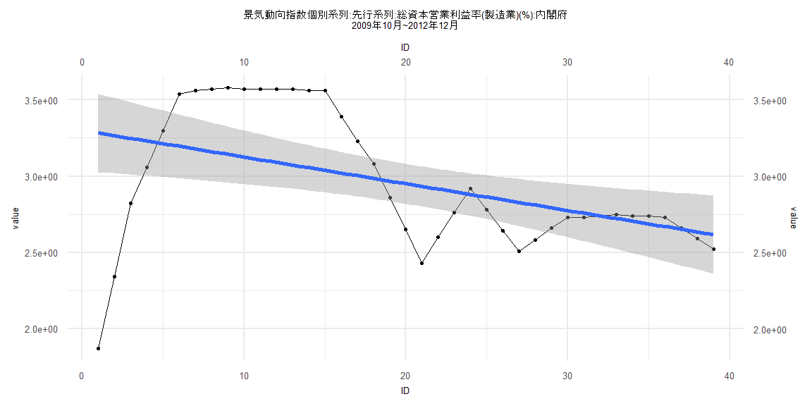
Call:
lm(formula = value ~ ID)

Residuals:
     Min       1Q   Median       3Q      Max
-1.41341 -0.15423  0.00783  0.35693  0.52207

Coefficients:
             Estimate Std. Error t value             Pr(>|t|)
(Intercept)  3.300945   0.131782  25.048 < 0.0000000000000002 ***
ID          -0.017534   0.005742  -3.054              0.00418 **
---
Signif. codes:  0 '***' 0.001 '**' 0.01 '*' 0.05 '.' 0.1 ' ' 1

Residual standard error: 0.4036 on 37 degrees of freedom
Multiple R-squared:  0.2013,    Adjusted R-squared:  0.1797
F-statistic: 9.324 on 1 and 37 DF,  p-value: 0.004175


    Two-sample Kolmogorov-Smirnov test

data:  lm_residuals and rnorm(n = length(lm_residuals), mean = 0, sd = sd(lm_residuals))
D = 0.12821, p-value = 0.9114
alternative hypothesis: two-sided


    Durbin-Watson test

data:  value ~ ID
DW = 0.17335, p-value < 0.00000000000000022
alternative hypothesis: true autocorrelation is greater than 0


    studentized Breusch-Pagan test

data:  value ~ ID
BP = 9.6928, df = 1, p-value = 0.00185


    Box-Ljung test

data:  lm_residuals
X-squared = 23.469, df = 1, p-value = 0.00000127
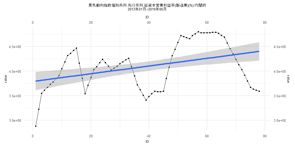
Call:
lm(formula = value ~ ID)

Residuals:
     Min       1Q   Median       3Q      Max
-0.91806 -0.31783  0.06303  0.39466  0.56369

Coefficients:
            Estimate Std. Error t value             Pr(>|t|)
(Intercept) 3.790233   0.096620  39.228 < 0.0000000000000002 ***
ID          0.007826   0.002125   3.683              0.00043 ***
---
Signif. codes:  0 '***' 0.001 '**' 0.01 '*' 0.05 '.' 0.1 ' ' 1

Residual standard error: 0.4226 on 76 degrees of freedom
Multiple R-squared:  0.1514,    Adjusted R-squared:  0.1403
F-statistic: 13.56 on 1 and 76 DF,  p-value: 0.0004297


    Two-sample Kolmogorov-Smirnov test

data:  lm_residuals and rnorm(n = length(lm_residuals), mean = 0, sd = sd(lm_residuals))
D = 0.12821, p-value = 0.546
alternative hypothesis: two-sided


    Durbin-Watson test

data:  value ~ ID
DW = 0.089451, p-value < 0.00000000000000022
alternative hypothesis: true autocorrelation is greater than 0


    studentized Breusch-Pagan test

data:  value ~ ID
BP = 8.7901, df = 1, p-value = 0.003029


    Box-Ljung test

data:  lm_residuals
X-squared = 65.643, df = 1, p-value = 0.0000000000000005551
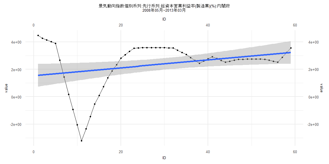
Call:
lm(formula = value ~ ID)

Residuals:
    Min      1Q  Median      3Q     Max
-5.0609 -0.2957  0.0154  1.1183  2.9071

Coefficients:
            Estimate Std. Error t value Pr(>|t|)
(Intercept)  1.53406    0.42248   3.631 0.000606 ***
ID           0.02880    0.01225   2.352 0.022162 *
---
Signif. codes:  0 '***' 0.001 '**' 0.01 '*' 0.05 '.' 0.1 ' ' 1

Residual standard error: 1.602 on 57 degrees of freedom
Multiple R-squared:  0.08845,   Adjusted R-squared:  0.07246
F-statistic: 5.531 on 1 and 57 DF,  p-value: 0.02216


    Two-sample Kolmogorov-Smirnov test

data:  lm_residuals and rnorm(n = length(lm_residuals), mean = 0, sd = sd(lm_residuals))
D = 0.16949, p-value = 0.3674
alternative hypothesis: two-sided


    Durbin-Watson test

data:  value ~ ID
DW = 0.094483, p-value < 0.00000000000000022
alternative hypothesis: true autocorrelation is greater than 0


    studentized Breusch-Pagan test

data:  value ~ ID
BP = 17.888, df = 1, p-value = 0.00002343


    Box-Ljung test

data:  lm_residuals
X-squared = 52.924, df = 1, p-value = 0.0000000000003467
Call:
lm(formula = value ~ ID)

Residuals:
     Min       1Q   Median       3Q      Max
-0.76097 -0.30221  0.05164  0.39087  0.57180

Coefficients:
            Estimate Std. Error t value             Pr(>|t|)
(Intercept) 3.912515   0.095110  41.137 < 0.0000000000000002 ***
ID          0.005846   0.002175   2.688              0.00889 **
---
Signif. codes:  0 '***' 0.001 '**' 0.01 '*' 0.05 '.' 0.1 ' ' 1

Residual standard error: 0.4077 on 73 degrees of freedom
Multiple R-squared:  0.09007,   Adjusted R-squared:  0.07761
F-statistic: 7.226 on 1 and 73 DF,  p-value: 0.008894


    Two-sample Kolmogorov-Smirnov test

data:  lm_residuals and rnorm(n = length(lm_residuals), mean = 0, sd = sd(lm_residuals))
D = 0.13333, p-value = 0.5204
alternative hypothesis: two-sided


    Durbin-Watson test

data:  value ~ ID
DW = 0.081987, p-value < 0.00000000000000022
alternative hypothesis: true autocorrelation is greater than 0


    studentized Breusch-Pagan test

data:  value ~ ID
BP = 19.629, df = 1, p-value = 0.000009403


    Box-Ljung test

data:  lm_residuals
X-squared = 67.676, df = 1, p-value = 0.000000000000000222