Analysis
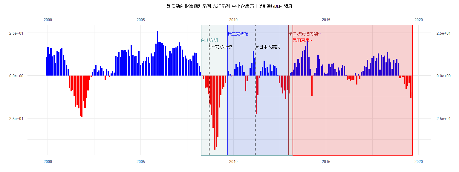
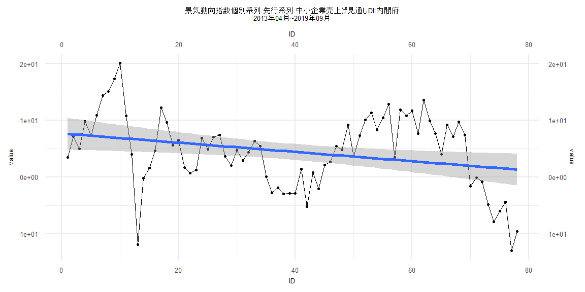
[1] "景気動向指数個別系列:先行系列:中小企業売上げ見通しDI:内閣府"
       Jan   Feb   Mar   Apr   May   Jun   Jul   Aug   Sep   Oct   Nov   Dec
1999                                                                    10.9
2000  16.7  12.6  16.1  11.2  12.3   7.4  14.1  13.8  15.8  16.0  11.9   9.0
2001   6.2   3.7  -7.4  -9.2  -8.4 -11.9 -18.2 -17.4 -19.2 -23.7 -24.4 -15.0
2002 -19.1 -12.9  -8.8  -2.6  -0.9   2.2   3.6   6.1   2.0   3.0   5.8   4.5
2003   2.6  -2.5   3.7   2.5  -0.8   1.2   2.4   1.7  11.3  11.0  13.6  10.9
2004  14.9  14.6  15.1  13.6  15.2  11.3  17.8  11.8  11.1  11.5   7.5  14.5
2005   6.2   7.3   8.4   8.8  11.0  10.7   7.3  12.9  11.1  13.6  18.7  26.2
2006  19.8  19.8  19.0  17.6  17.5  11.7  10.4  14.4  12.9  16.3  16.1  16.4
2007  17.4  19.4  17.5  15.2  10.6  11.7   9.9   9.2   9.5   8.4  11.7  13.4
2008  13.1   7.4   5.7   2.1  -0.3  -1.9  -7.5  -7.0 -11.1 -17.0 -22.9 -30.6
2009 -43.3 -41.9 -36.0 -18.8 -11.6  -8.1  -6.7  -4.4   0.0   2.8   0.7  -0.5
2010  -0.4   3.9   6.6   5.1   8.0   5.6   5.9   1.9  -9.3  -3.3  -0.3   4.4
2011   7.1  14.2  10.5 -22.5 -11.5  -1.3   2.7   5.1   8.8   4.6   5.1   1.7
2012   6.4   2.4   6.3   5.7   4.4   0.4  -4.6  -7.0 -10.5  -8.8 -13.8  -8.5
2013 -10.5   1.3   2.0   3.5   7.1   5.0   9.8   7.3  10.9  14.4  15.1  17.3
2014  20.1  10.8   4.0 -11.9  -0.2   1.6   4.6  12.2   9.6   5.6   6.5   1.7
2015   0.7   1.2   6.9   4.9   7.0   7.4   3.6   2.0   4.7   2.9   4.4   6.3
2016   5.4   0.1  -2.8  -1.9  -3.0  -2.9  -2.9   1.4  -5.2   0.8  -2.1   2.1
2017   2.7   5.4   4.8   9.2   3.6   7.3  10.1  11.3   8.3  10.4  12.9   3.5
2018  11.9  10.8  11.7   7.7  13.6   9.9   7.7   4.0   9.2   7.1   9.7   7.4
2019  -1.6  -0.1  -0.8  -4.9  -7.9  -6.0  -4.4 -13.0  -9.6
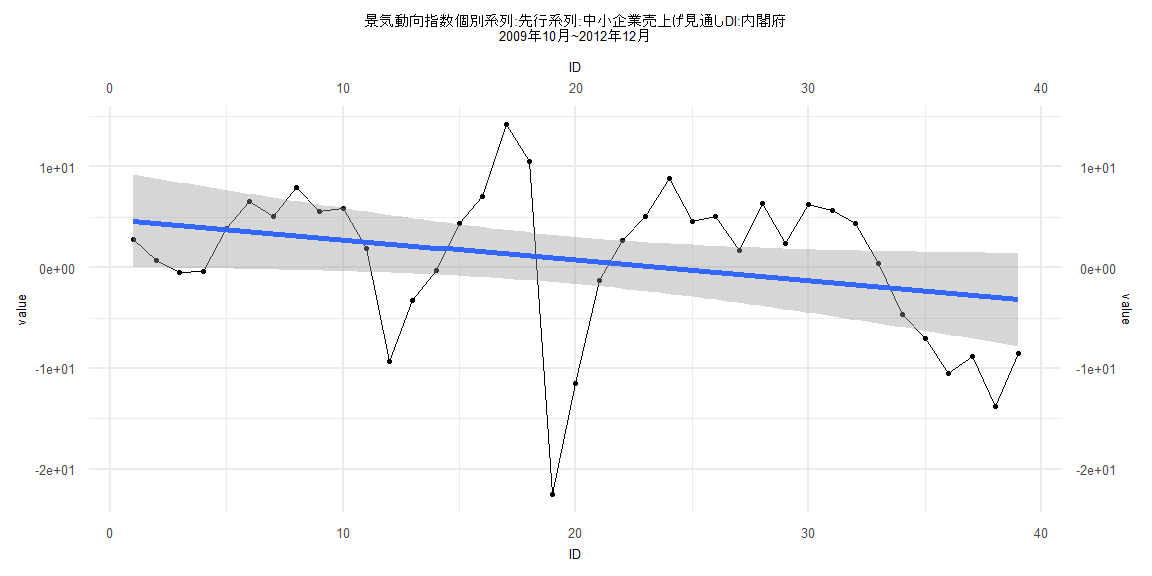
Call:
lm(formula = value ~ ID)

Residuals:
    Min      1Q  Median      3Q     Max
-23.423  -4.521   2.351   4.953  12.866

Coefficients:
            Estimate Std. Error t value Pr(>|t|)
(Intercept)   4.8244     2.3631   2.042   0.0484 *
ID           -0.2053     0.1030  -1.994   0.0536 .
---
Signif. codes:  0 '***' 0.001 '**' 0.01 '*' 0.05 '.' 0.1 ' ' 1

Residual standard error: 7.237 on 37 degrees of freedom
Multiple R-squared:  0.09703,   Adjusted R-squared:  0.07263
F-statistic: 3.976 on 1 and 37 DF,  p-value: 0.05356


    Two-sample Kolmogorov-Smirnov test

data:  lm_residuals and rnorm(n = length(lm_residuals), mean = 0, sd = sd(lm_residuals))
D = 0.20513, p-value = 0.3888
alternative hypothesis: two-sided


    Durbin-Watson test

data:  value ~ ID
DW = 0.96713, p-value = 0.0001105
alternative hypothesis: true autocorrelation is greater than 0


    studentized Breusch-Pagan test

data:  value ~ ID
BP = 0.27095, df = 1, p-value = 0.6027


    Box-Ljung test

data:  lm_residuals
X-squared = 10.871, df = 1, p-value = 0.0009766
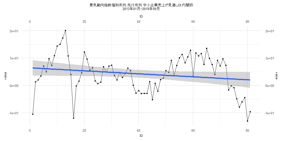
Call:
lm(formula = value ~ ID)

Residuals:
     Min       1Q   Median       3Q      Max
-17.4722  -4.0577   0.0567   4.9145  14.3639

Coefficients:
            Estimate Std. Error t value  Pr(>|t|)
(Intercept)  6.44645    1.46014   4.415 0.0000317 ***
ID          -0.05464    0.03094  -1.766    0.0812 .
---
Signif. codes:  0 '***' 0.001 '**' 0.01 '*' 0.05 '.' 0.1 ' ' 1

Residual standard error: 6.51 on 79 degrees of freedom
Multiple R-squared:  0.03799,   Adjusted R-squared:  0.02581
F-statistic:  3.12 on 1 and 79 DF,  p-value: 0.08122


    Two-sample Kolmogorov-Smirnov test

data:  lm_residuals and rnorm(n = length(lm_residuals), mean = 0, sd = sd(lm_residuals))
D = 0.08642, p-value = 0.9254
alternative hypothesis: two-sided


    Durbin-Watson test

data:  value ~ ID
DW = 0.50647, p-value < 0.00000000000000022
alternative hypothesis: true autocorrelation is greater than 0


    studentized Breusch-Pagan test

data:  value ~ ID
BP = 0.064866, df = 1, p-value = 0.799


    Box-Ljung test

data:  lm_residuals
X-squared = 39.316, df = 1, p-value = 0.0000000003605
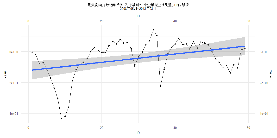
Call:
lm(formula = value ~ ID)

Residuals:
    Min      1Q  Median      3Q     Max
-33.467  -6.190   3.558   7.773  17.337

Coefficients:
            Estimate Std. Error t value Pr(>|t|)
(Intercept) -12.2441     3.0324  -4.038 0.000163 ***
ID            0.2679     0.0879   3.047 0.003498 **
---
Signif. codes:  0 '***' 0.001 '**' 0.01 '*' 0.05 '.' 0.1 ' ' 1

Residual standard error: 11.5 on 57 degrees of freedom
Multiple R-squared:  0.1401,    Adjusted R-squared:  0.125
F-statistic: 9.285 on 1 and 57 DF,  p-value: 0.003498


    Two-sample Kolmogorov-Smirnov test

data:  lm_residuals and rnorm(n = length(lm_residuals), mean = 0, sd = sd(lm_residuals))
D = 0.10169, p-value = 0.9239
alternative hypothesis: two-sided


    Durbin-Watson test

data:  value ~ ID
DW = 0.37106, p-value < 0.00000000000000022
alternative hypothesis: true autocorrelation is greater than 0


    studentized Breusch-Pagan test

data:  value ~ ID
BP = 3.8151, df = 1, p-value = 0.05079


    Box-Ljung test

data:  lm_residuals
X-squared = 40.237, df = 1, p-value = 0.0000000002249
Call:
lm(formula = value ~ ID)

Residuals:
     Min       1Q   Median       3Q      Max
-18.5282  -4.2327  -0.2147   5.0191  13.2264

Coefficients:
            Estimate Std. Error t value    Pr(>|t|)
(Intercept)  7.69167    1.43198   5.371 0.000000824 ***
ID          -0.08181    0.03150  -2.597      0.0113 *
---
Signif. codes:  0 '***' 0.001 '**' 0.01 '*' 0.05 '.' 0.1 ' ' 1

Residual standard error: 6.263 on 76 degrees of freedom
Multiple R-squared:  0.08153,   Adjusted R-squared:  0.06945
F-statistic: 6.747 on 1 and 76 DF,  p-value: 0.01127


    Two-sample Kolmogorov-Smirnov test

data:  lm_residuals and rnorm(n = length(lm_residuals), mean = 0, sd = sd(lm_residuals))
D = 0.089744, p-value = 0.9147
alternative hypothesis: two-sided


    Durbin-Watson test

data:  value ~ ID
DW = 0.52054, p-value = 0.0000000000000005029
alternative hypothesis: true autocorrelation is greater than 0


    studentized Breusch-Pagan test

data:  value ~ ID
BP = 1.2555, df = 1, p-value = 0.2625


    Box-Ljung test

data:  lm_residuals
X-squared = 41.653, df = 1, p-value = 0.000000000109