Analysis
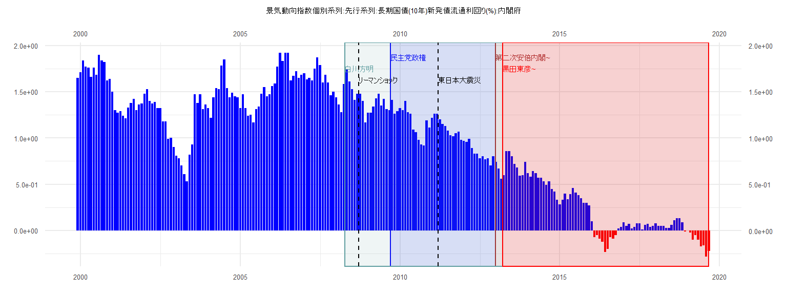
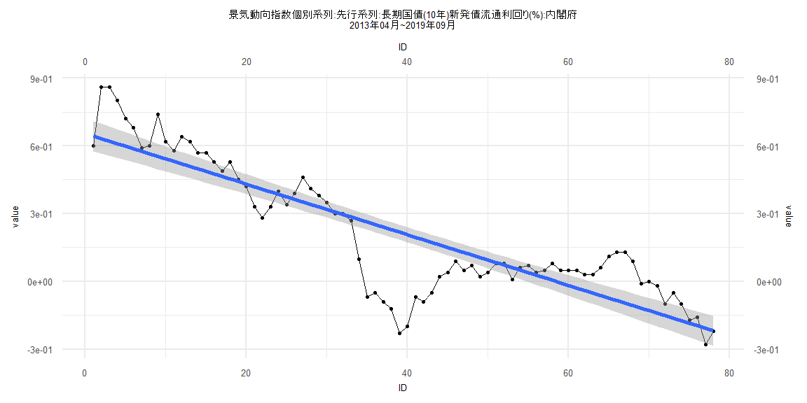
[1] "景気動向指数個別系列:先行系列:長期国債(10年)新発債流通利回り(%):内閣府"
       Jan   Feb   Mar   Apr   May   Jun   Jul   Aug   Sep   Oct   Nov   Dec
1999                                                                    1.65
2000  1.71  1.84  1.77  1.76  1.66  1.76  1.68  1.90  1.84  1.82  1.62  1.64
2001  1.50  1.30  1.27  1.29  1.24  1.21  1.33  1.38  1.42  1.30  1.36  1.37
2002  1.48  1.53  1.40  1.37  1.39  1.32  1.32  1.18  1.18  0.99  1.00  0.90
2003  0.81  0.78  0.70  0.61  0.53  0.82  0.93  1.47  1.38  1.47  1.31  1.36
2004  1.32  1.22  1.44  1.54  1.53  1.78  1.85  1.54  1.44  1.49  1.45  1.44
2005  1.32  1.47  1.32  1.24  1.25  1.17  1.31  1.34  1.48  1.55  1.45  1.47
2006  1.56  1.59  1.77  1.92  1.83  1.92  1.92  1.62  1.67  1.72  1.65  1.68
2007  1.70  1.63  1.65  1.62  1.75  1.87  1.79  1.60  1.68  1.60  1.46  1.50
2008  1.44  1.36  1.28  1.58  1.74  1.61  1.53  1.41  1.48  1.48  1.40  1.17
2009  1.27  1.27  1.34  1.43  1.48  1.35  1.42  1.31  1.30  1.41  1.26  1.29
2010  1.32  1.30  1.40  1.28  1.26  1.09  1.06  0.98  0.93  0.92  1.19  1.11
2011  1.22  1.26  1.26  1.20  1.15  1.13  1.08  1.03  1.02  1.05  1.07  0.98
2012  0.97  0.96  0.99  0.89  0.83  0.83  0.78  0.80  0.77  0.78  0.70  0.80
2013  0.74  0.67  0.56  0.60  0.86  0.86  0.80  0.72  0.68  0.59  0.60  0.74
2014  0.62  0.58  0.64  0.62  0.57  0.57  0.53  0.49  0.53  0.45  0.42  0.33
2015  0.28  0.33  0.40  0.34  0.39  0.46  0.41  0.38  0.35  0.30  0.30  0.27
2016  0.10 -0.07 -0.05 -0.09 -0.12 -0.23 -0.20 -0.07 -0.09 -0.05  0.02  0.04
2017  0.09  0.05  0.07  0.02  0.04  0.08  0.08  0.01  0.06  0.07  0.04  0.05
2018  0.08  0.05  0.05  0.05  0.03  0.03  0.06  0.11  0.13  0.13  0.09 -0.01
2019  0.00 -0.02 -0.10 -0.05 -0.10 -0.17 -0.16 -0.28 -0.22
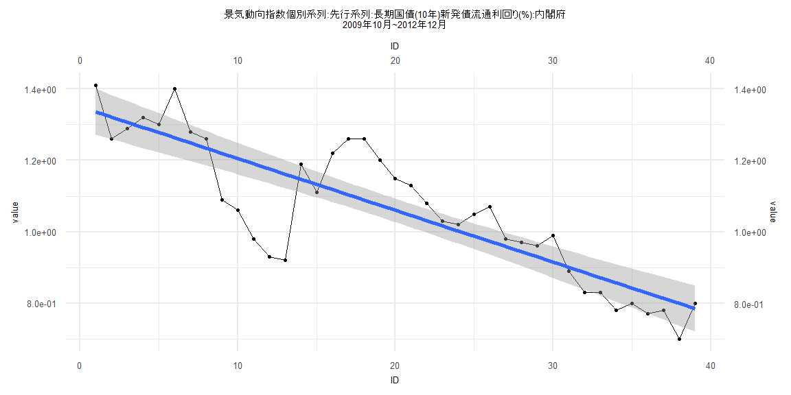
Call:
lm(formula = value ~ ID)

Residuals:
     Min       1Q   Median       3Q      Max
-0.24622 -0.04956  0.02122  0.06827  0.17075

Coefficients:
             Estimate Std. Error t value             Pr(>|t|)
(Intercept)  1.350175   0.033127   40.76 < 0.0000000000000002 ***
ID          -0.014496   0.001443  -10.04     0.00000000000409 ***
---
Signif. codes:  0 '***' 0.001 '**' 0.01 '*' 0.05 '.' 0.1 ' ' 1

Residual standard error: 0.1015 on 37 degrees of freedom
Multiple R-squared:  0.7316,    Adjusted R-squared:  0.7243
F-statistic: 100.9 on 1 and 37 DF,  p-value: 0.000000000004088


    Two-sample Kolmogorov-Smirnov test

data:  lm_residuals and rnorm(n = length(lm_residuals), mean = 0, sd = sd(lm_residuals))
D = 0.15385, p-value = 0.7523
alternative hypothesis: two-sided


    Durbin-Watson test

data:  value ~ ID
DW = 0.59762, p-value = 0.00000003614
alternative hypothesis: true autocorrelation is greater than 0


    studentized Breusch-Pagan test

data:  value ~ ID
BP = 2.8814, df = 1, p-value = 0.08961


    Box-Ljung test

data:  lm_residuals
X-squared = 20.245, df = 1, p-value = 0.000006812
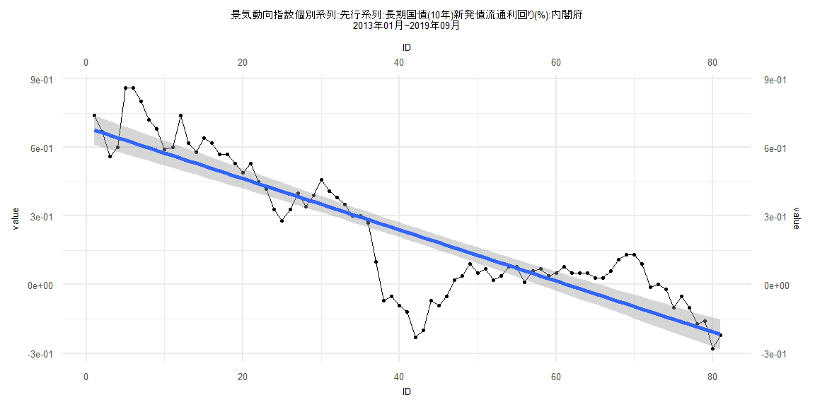
Call:
lm(formula = value ~ ID)

Residuals:
     Min       1Q   Median       3Q      Max
-0.44759 -0.05113  0.02712  0.07831  0.24008

Coefficients:
              Estimate Std. Error t value            Pr(>|t|)
(Intercept)  0.6869784  0.0328625   20.91 <0.0000000000000002 ***
ID          -0.0111759  0.0006963  -16.05 <0.0000000000000002 ***
---
Signif. codes:  0 '***' 0.001 '**' 0.01 '*' 0.05 '.' 0.1 ' ' 1

Residual standard error: 0.1465 on 79 degrees of freedom
Multiple R-squared:  0.7653,    Adjusted R-squared:  0.7624
F-statistic: 257.6 on 1 and 79 DF,  p-value: < 0.00000000000000022


    Two-sample Kolmogorov-Smirnov test

data:  lm_residuals and rnorm(n = length(lm_residuals), mean = 0, sd = sd(lm_residuals))
D = 0.18519, p-value = 0.1245
alternative hypothesis: two-sided


    Durbin-Watson test

data:  value ~ ID
DW = 0.20835, p-value < 0.00000000000000022
alternative hypothesis: true autocorrelation is greater than 0


    studentized Breusch-Pagan test

data:  value ~ ID
BP = 0.0021399, df = 1, p-value = 0.9631


    Box-Ljung test

data:  lm_residuals
X-squared = 67.257, df = 1, p-value = 0.000000000000000222
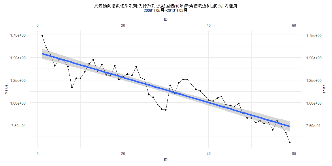
Call:
lm(formula = value ~ ID)

Residuals:
     Min       1Q   Median       3Q      Max
-0.27651 -0.05585  0.01022  0.06747  0.19624

Coefficients:
              Estimate Std. Error t value            Pr(>|t|)
(Intercept)  1.5576563  0.0278894   55.85 <0.0000000000000002 ***
ID          -0.0138936  0.0008085  -17.18 <0.0000000000000002 ***
---
Signif. codes:  0 '***' 0.001 '**' 0.01 '*' 0.05 '.' 0.1 ' ' 1

Residual standard error: 0.1058 on 57 degrees of freedom
Multiple R-squared:  0.8382,    Adjusted R-squared:  0.8354
F-statistic: 295.3 on 1 and 57 DF,  p-value: < 0.00000000000000022


    Two-sample Kolmogorov-Smirnov test

data:  lm_residuals and rnorm(n = length(lm_residuals), mean = 0, sd = sd(lm_residuals))
D = 0.11864, p-value = 0.8052
alternative hypothesis: two-sided


    Durbin-Watson test

data:  value ~ ID
DW = 0.64287, p-value = 0.0000000002498
alternative hypothesis: true autocorrelation is greater than 0


    studentized Breusch-Pagan test

data:  value ~ ID
BP = 1.6368, df = 1, p-value = 0.2008


    Box-Ljung test

data:  lm_residuals
X-squared = 24.125, df = 1, p-value = 0.0000009029
Call:
lm(formula = value ~ ID)

Residuals:
     Min       1Q   Median       3Q      Max
-0.44791 -0.05075  0.02889  0.08021  0.23902

Coefficients:
              Estimate Std. Error t value            Pr(>|t|)
(Intercept)  0.6545654  0.0340251   19.24 <0.0000000000000002 ***
ID          -0.0111964  0.0007484  -14.96 <0.0000000000000002 ***
---
Signif. codes:  0 '***' 0.001 '**' 0.01 '*' 0.05 '.' 0.1 ' ' 1

Residual standard error: 0.1488 on 76 degrees of freedom
Multiple R-squared:  0.7465,    Adjusted R-squared:  0.7432
F-statistic: 223.8 on 1 and 76 DF,  p-value: < 0.00000000000000022


    Two-sample Kolmogorov-Smirnov test

data:  lm_residuals and rnorm(n = length(lm_residuals), mean = 0, sd = sd(lm_residuals))
D = 0.12821, p-value = 0.546
alternative hypothesis: two-sided


    Durbin-Watson test

data:  value ~ ID
DW = 0.20054, p-value < 0.00000000000000022
alternative hypothesis: true autocorrelation is greater than 0


    studentized Breusch-Pagan test

data:  value ~ ID
BP = 0.090455, df = 1, p-value = 0.7636


    Box-Ljung test

data:  lm_residuals
X-squared = 65.521, df = 1, p-value = 0.0000000000000005551