Analysis
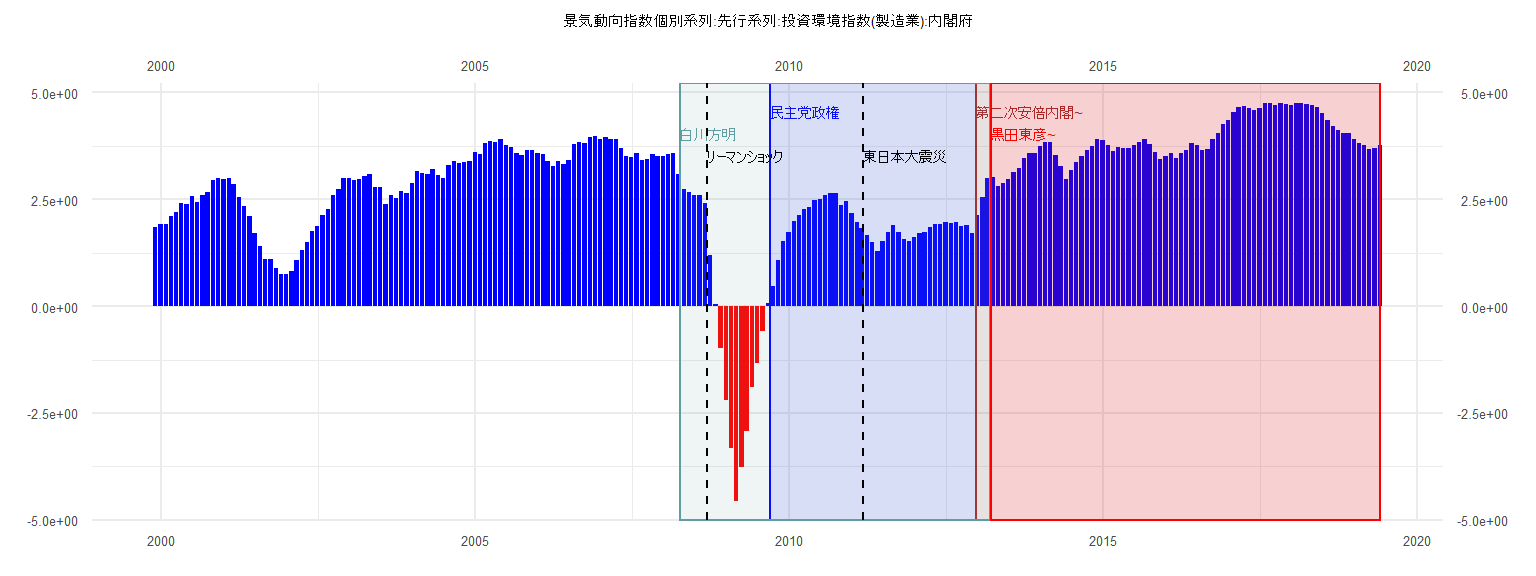
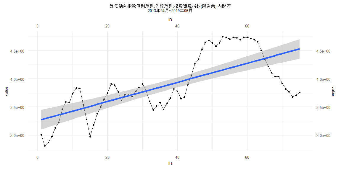
[1] "景気動向指数個別系列:先行系列:投資環境指数(製造業):内閣府"
       Jan   Feb   Mar   Apr   May   Jun   Jul   Aug   Sep   Oct   Nov   Dec
1999                                                                    1.86
2000  1.92  1.92  2.11  2.21  2.40  2.39  2.57  2.44  2.59  2.67  2.94  3.00
2001  2.98  3.00  2.86  2.55  2.34  2.10  1.72  1.41  1.10  1.09  0.90  0.76
2002  0.76  0.83  1.08  1.31  1.49  1.75  1.87  2.14  2.27  2.61  2.75  2.99
2003  3.00  2.96  2.97  3.05  3.10  2.79  2.79  2.38  2.60  2.53  2.70  2.65
2004  2.88  3.15  3.11  3.10  3.21  3.07  3.00  3.30  3.39  3.34  3.38  3.39
2005  3.61  3.56  3.81  3.86  3.83  3.90  3.76  3.72  3.57  3.53  3.65  3.65
2006  3.57  3.56  3.40  3.27  3.39  3.33  3.42  3.80  3.83  3.82  3.95  3.97
2007  3.92  3.95  3.90  3.90  3.70  3.52  3.49  3.59  3.42  3.45  3.56  3.50
2008  3.51  3.55  3.59  3.09  2.73  2.66  2.61  2.61  2.41  1.19  0.04 -0.99
2009 -2.19 -3.32 -4.55 -3.77 -2.92 -1.89 -1.33 -0.58  0.08  0.46  1.08  1.53
2010  1.74  2.00  2.14  2.28  2.31  2.49  2.51  2.59  2.64  2.65  2.37  2.45
2011  2.17  1.97  1.82  1.66  1.50  1.30  1.52  1.73  1.90  1.73  1.57  1.53
2012  1.61  1.70  1.74  1.84  1.91  1.92  1.96  1.94  1.96  1.88  1.89  1.72
2013  2.14  2.55  2.99  3.01  2.81  2.87  2.98  3.13  3.23  3.46  3.59  3.58
2014  3.74  3.84  3.83  3.54  3.28  2.97  3.18  3.38  3.50  3.64  3.75  3.91
2015  3.89  3.77  3.62  3.72  3.71  3.69  3.78  3.85  3.91  3.79  3.60  3.45
2016  3.52  3.58  3.46  3.57  3.66  3.82  3.78  3.65  3.68  3.90  4.06  4.27
2017  4.35  4.53  4.65  4.68  4.64  4.58  4.64  4.75  4.74  4.71  4.74  4.73
2018  4.70  4.74  4.74  4.72  4.70  4.66  4.51  4.35  4.22  4.11  4.04  4.04
2019  3.92  3.82  3.77  3.68  3.71  3.76
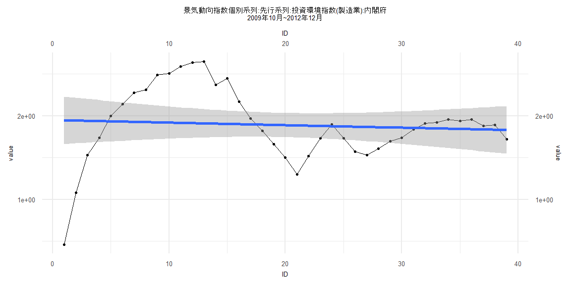
Call:
lm(formula = value ~ ID)

Residuals:
     Min       1Q   Median       3Q      Max
-1.48773 -0.21583  0.04165  0.23765  0.73873

Coefficients:
             Estimate Std. Error t value             Pr(>|t|)
(Intercept)  1.950769   0.145768  13.383 0.000000000000000942 ***
ID          -0.003038   0.006352  -0.478                0.635
---
Signif. codes:  0 '***' 0.001 '**' 0.01 '*' 0.05 '.' 0.1 ' ' 1

Residual standard error: 0.4464 on 37 degrees of freedom
Multiple R-squared:  0.006147,  Adjusted R-squared:  -0.02071
F-statistic: 0.2288 on 1 and 37 DF,  p-value: 0.6352


    Two-sample Kolmogorov-Smirnov test

data:  lm_residuals and rnorm(n = length(lm_residuals), mean = 0, sd = sd(lm_residuals))
D = 0.25641, p-value = 0.1547
alternative hypothesis: two-sided


    Durbin-Watson test

data:  value ~ ID
DW = 0.18332, p-value < 0.00000000000000022
alternative hypothesis: true autocorrelation is greater than 0


    studentized Breusch-Pagan test

data:  value ~ ID
BP = 9.5451, df = 1, p-value = 0.002005


    Box-Ljung test

data:  lm_residuals
X-squared = 24.14, df = 1, p-value = 0.000000896
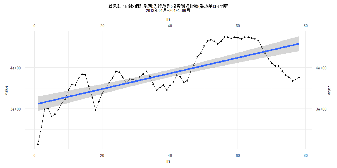
Call:
lm(formula = value ~ ID)

Residuals:
     Min       1Q   Median       3Q      Max
-0.98332 -0.28288  0.02888  0.34206  0.58965

Coefficients:
            Estimate Std. Error t value             Pr(>|t|)
(Intercept) 3.104362   0.091621  33.883 < 0.0000000000000002 ***
ID          0.018961   0.002015   9.409    0.000000000000022 ***
---
Signif. codes:  0 '***' 0.001 '**' 0.01 '*' 0.05 '.' 0.1 ' ' 1

Residual standard error: 0.4007 on 76 degrees of freedom
Multiple R-squared:  0.5381,    Adjusted R-squared:  0.532
F-statistic: 88.54 on 1 and 76 DF,  p-value: 0.00000000000002202


    Two-sample Kolmogorov-Smirnov test

data:  lm_residuals and rnorm(n = length(lm_residuals), mean = 0, sd = sd(lm_residuals))
D = 0.089744, p-value = 0.9147
alternative hypothesis: two-sided


    Durbin-Watson test

data:  value ~ ID
DW = 0.1206, p-value < 0.00000000000000022
alternative hypothesis: true autocorrelation is greater than 0


    studentized Breusch-Pagan test

data:  value ~ ID
BP = 10.082, df = 1, p-value = 0.001497


    Box-Ljung test

data:  lm_residuals
X-squared = 61.664, df = 1, p-value = 0.000000000000004108
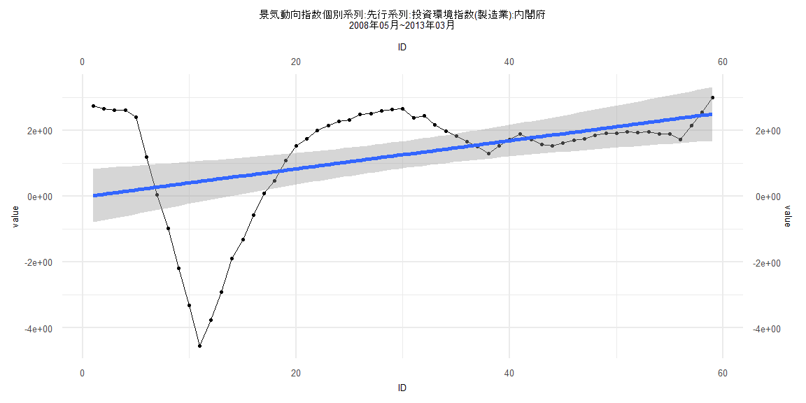
Call:
lm(formula = value ~ ID)

Residuals:
    Min      1Q  Median      3Q     Max
-4.9961 -0.2933 -0.0562  1.0771  2.7109

Coefficients:
            Estimate Std. Error t value Pr(>|t|)
(Intercept) -0.02359    0.41859  -0.056  0.95525
ID           0.04270    0.01213   3.519  0.00086 ***
---
Signif. codes:  0 '***' 0.001 '**' 0.01 '*' 0.05 '.' 0.1 ' ' 1

Residual standard error: 1.587 on 57 degrees of freedom
Multiple R-squared:  0.1784,    Adjusted R-squared:  0.164
F-statistic: 12.38 on 1 and 57 DF,  p-value: 0.0008598


    Two-sample Kolmogorov-Smirnov test

data:  lm_residuals and rnorm(n = length(lm_residuals), mean = 0, sd = sd(lm_residuals))
D = 0.25424, p-value = 0.04374
alternative hypothesis: two-sided


    Durbin-Watson test

data:  value ~ ID
DW = 0.097231, p-value < 0.00000000000000022
alternative hypothesis: true autocorrelation is greater than 0


    studentized Breusch-Pagan test

data:  value ~ ID
BP = 17.43, df = 1, p-value = 0.0000298


    Box-Ljung test

data:  lm_residuals
X-squared = 53.087, df = 1, p-value = 0.0000000000003192
Call:
lm(formula = value ~ ID)

Residuals:
     Min       1Q   Median       3Q      Max
-0.82007 -0.29057  0.00893  0.32043  0.58993

Coefficients:
            Estimate Std. Error t value             Pr(>|t|)
(Intercept)  3.25907    0.08922  36.527 < 0.0000000000000002 ***
ID           0.01700    0.00204   8.333     0.00000000000333 ***
---
Signif. codes:  0 '***' 0.001 '**' 0.01 '*' 0.05 '.' 0.1 ' ' 1

Residual standard error: 0.3825 on 73 degrees of freedom
Multiple R-squared:  0.4875,    Adjusted R-squared:  0.4805
F-statistic: 69.44 on 1 and 73 DF,  p-value: 0.000000000003335


    Two-sample Kolmogorov-Smirnov test

data:  lm_residuals and rnorm(n = length(lm_residuals), mean = 0, sd = sd(lm_residuals))
D = 0.14667, p-value = 0.3974
alternative hypothesis: two-sided


    Durbin-Watson test

data:  value ~ ID
DW = 0.10667, p-value < 0.00000000000000022
alternative hypothesis: true autocorrelation is greater than 0


    studentized Breusch-Pagan test

data:  value ~ ID
BP = 22.822, df = 1, p-value = 0.000001777


    Box-Ljung test

data:  lm_residuals
X-squared = 65.38, df = 1, p-value = 0.0000000000000006661