Analysis
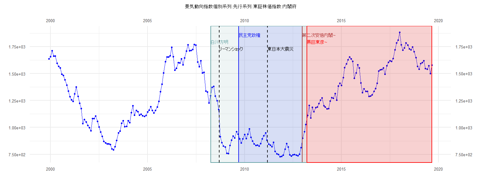
[1] "景気動向指数個別系列:先行系列:東証株価指数:内閣府"
Jan Feb Mar Apr May Jun Jul Aug Sep Oct Nov Dec
1999 1637.52
2000 1657.91 1711.97 1661.73 1661.89 1595.11 1566.27 1552.98 1493.44 1483.96 1443.34 1392.39 1336.78
2001 1284.67 1257.92 1240.74 1311.51 1376.04 1289.61 1224.91 1174.71 1035.73 1072.61 1050.44 1018.09
2002 999.01 970.11 1083.89 1083.27 1105.87 1056.54 1003.17 956.43 916.01 871.56 856.11 847.24
2003 847.86 841.75 802.14 791.55 820.42 879.19 949.44 965.77 1038.26 1062.92 1007.04 1010.30
2004 1061.40 1045.70 1137.66 1200.99 1113.85 1158.74 1146.49 1114.78 1122.40 1108.48 1101.78 1110.39
2005 1144.09 1159.71 1191.82 1158.22 1134.29 1159.35 1189.41 1241.61 1333.02 1400.34 1505.63 1611.10
2006 1654.17 1653.33 1665.10 1745.00 1657.22 1532.82 1549.25 1601.79 1599.36 1635.35 1580.23 1646.40
2007 1708.42 1765.50 1711.78 1714.63 1724.49 1768.46 1762.62 1606.10 1562.37 1619.67 1504.90 1510.22
2008 1337.71 1328.42 1228.87 1294.08 1373.83 1380.74 1290.26 1247.10 1165.80 913.49 857.92 827.40
2009 819.66 762.16 756.52 832.63 882.40 921.57 903.66 961.13 937.02 895.10 855.14 892.90
2010 936.12 896.61 936.98 987.60 907.38 873.79 846.85 834.51 836.55 827.07 849.90 894.54
2011 924.36 948.61 883.59 843.89 837.02 822.06 861.29 778.73 753.81 750.34 730.12 732.53
2012 744.40 799.32 850.37 817.43 745.33 733.19 746.00 748.73 742.65 736.24 753.21 811.87
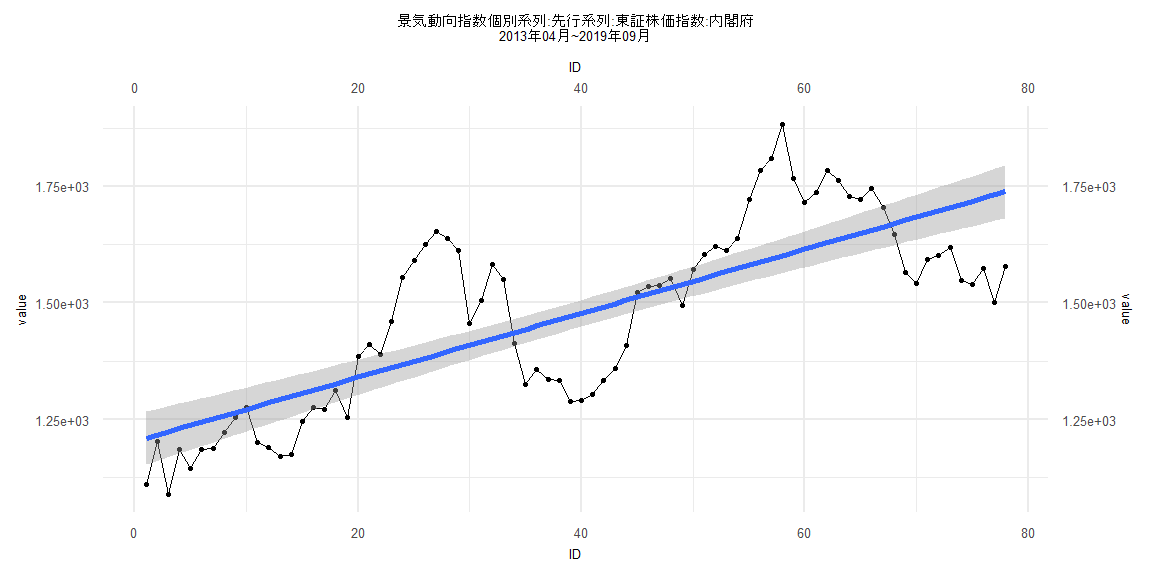
2013 901.20 961.02 1028.55 1110.41 1203.38 1089.48 1186.91 1145.42 1185.18 1188.51 1222.90 1254.45
2014 1275.17 1200.83 1190.57 1171.18 1174.62 1246.22 1275.72 1271.50 1313.29 1253.99 1385.33 1411.59
2015 1389.14 1461.08 1553.83 1590.91 1626.44 1652.72 1637.30 1613.59 1455.30 1506.15 1582.45 1551.34
2016 1412.22 1324.59 1358.30 1335.67 1334.43 1288.83 1291.30 1303.93 1334.42 1360.45 1409.47 1522.68
2017 1534.42 1537.60 1552.10 1494.81 1571.62 1603.77 1620.17 1612.95 1638.79 1721.72 1783.26 1809.61
2018 1882.57 1766.57 1716.27 1737.42 1783.96 1762.48 1729.12 1721.03 1746.41 1703.85 1646.77 1565.86
2019 1541.56 1592.61 1602.83 1618.12 1547.17 1540.08 1573.16 1501.08 1579.13
Call:
lm(formula = value ~ ID)

Residuals:
    Min      1Q  Median      3Q     Max
-70.246 -32.725  -8.491  32.812 103.942

Coefficients:
            Estimate Std. Error t value             Pr(>|t|)
(Intercept) 928.3506    14.8955  62.324 < 0.0000000000000002 ***
ID           -4.9225     0.6491  -7.584        0.00000000479 ***
---
Signif. codes:  0 '***' 0.001 '**' 0.01 '*' 0.05 '.' 0.1 ' ' 1

Residual standard error: 45.62 on 37 degrees of freedom
Multiple R-squared:  0.6085,    Adjusted R-squared:  0.598
F-statistic: 57.52 on 1 and 37 DF,  p-value: 0.000000004794


    Two-sample Kolmogorov-Smirnov test

data:  lm_residuals and rnorm(n = length(lm_residuals), mean = 0, sd = sd(lm_residuals))
D = 0.23077, p-value = 0.2523
alternative hypothesis: two-sided


    Durbin-Watson test

data:  value ~ ID
DW = 0.71325, p-value = 0.0000007913
alternative hypothesis: true autocorrelation is greater than 0


    studentized Breusch-Pagan test

data:  value ~ ID
BP = 0.051813, df = 1, p-value = 0.8199


    Box-Ljung test

data:  lm_residuals
X-squared = 15.207, df = 1, p-value = 0.00009636
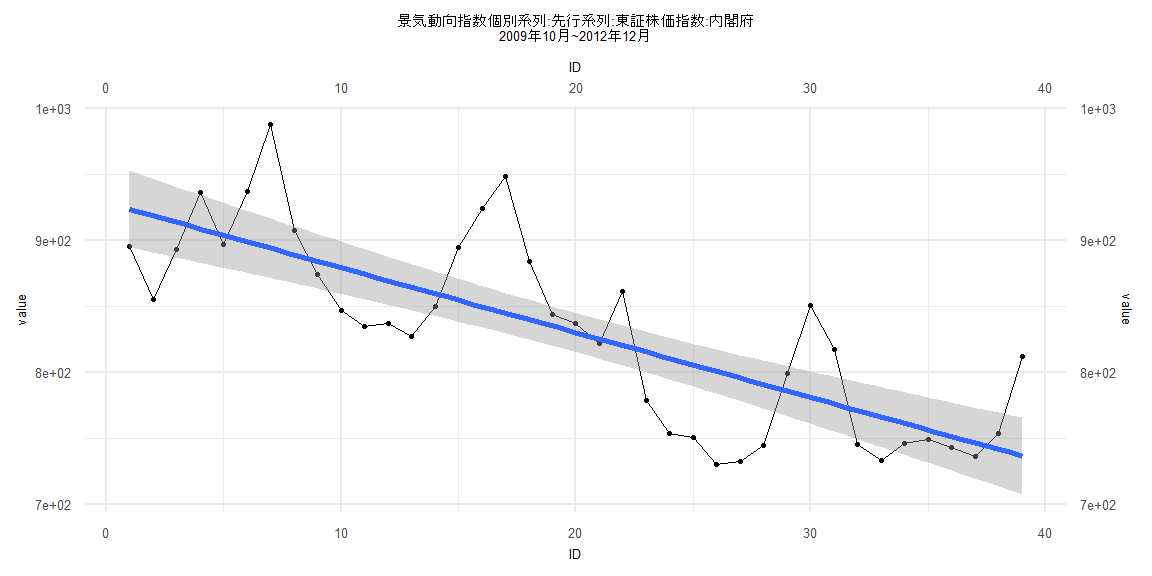
Call:
lm(formula = value ~ ID)

Residuals:
     Min       1Q   Median       3Q      Max
-254.728 -103.875   -7.882   81.475  279.716

Coefficients:
             Estimate Std. Error t value            Pr(>|t|)
(Intercept) 1148.4425    29.5645   38.84 <0.0000000000000002 ***
ID             7.4854     0.6264   11.95 <0.0000000000000002 ***
---
Signif. codes:  0 '***' 0.001 '**' 0.01 '*' 0.05 '.' 0.1 ' ' 1

Residual standard error: 131.8 on 79 degrees of freedom
Multiple R-squared:  0.6438,    Adjusted R-squared:  0.6393
F-statistic: 142.8 on 1 and 79 DF,  p-value: < 0.00000000000000022


    Two-sample Kolmogorov-Smirnov test

data:  lm_residuals and rnorm(n = length(lm_residuals), mean = 0, sd = sd(lm_residuals))
D = 0.1358, p-value = 0.4462
alternative hypothesis: two-sided


    Durbin-Watson test

data:  value ~ ID
DW = 0.19218, p-value < 0.00000000000000022
alternative hypothesis: true autocorrelation is greater than 0


    studentized Breusch-Pagan test

data:  value ~ ID
BP = 1.1069, df = 1, p-value = 0.2928


    Box-Ljung test

data:  lm_residuals
X-squared = 63.467, df = 1, p-value = 0.000000000000001665
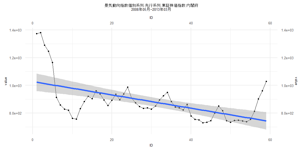
Call:
lm(formula = value ~ ID)

Residuals:
    Min      1Q  Median      3Q     Max
-217.65  -57.05  -28.31   21.46  363.33

Coefficients:
             Estimate Std. Error t value             Pr(>|t|)
(Intercept) 1027.0241    32.3765  31.721 < 0.0000000000000002 ***
ID            -4.8047     0.9385  -5.119           0.00000377 ***
---
Signif. codes:  0 '***' 0.001 '**' 0.01 '*' 0.05 '.' 0.1 ' ' 1

Residual standard error: 122.8 on 57 degrees of freedom
Multiple R-squared:  0.315, Adjusted R-squared:  0.3029
F-statistic: 26.21 on 1 and 57 DF,  p-value: 0.000003768


    Two-sample Kolmogorov-Smirnov test

data:  lm_residuals and rnorm(n = length(lm_residuals), mean = 0, sd = sd(lm_residuals))
D = 0.30508, p-value = 0.00792
alternative hypothesis: two-sided


    Durbin-Watson test

data:  value ~ ID
DW = 0.20081, p-value < 0.00000000000000022
alternative hypothesis: true autocorrelation is greater than 0


    studentized Breusch-Pagan test

data:  value ~ ID
BP = 8.6266, df = 1, p-value = 0.003313


    Box-Ljung test

data:  lm_residuals
X-squared = 37.788, df = 1, p-value = 0.0000000007887
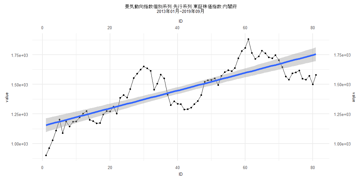
Call:
lm(formula = value ~ ID)

Residuals:
    Min      1Q  Median      3Q     Max
-230.75  -97.43  -13.30   89.25  281.25

Coefficients:
             Estimate Std. Error t value            Pr(>|t|)
(Intercept) 1202.9508    29.0501   41.41 <0.0000000000000002 ***
ID             6.8685     0.6389   10.75 <0.0000000000000002 ***
---
Signif. codes:  0 '***' 0.001 '**' 0.01 '*' 0.05 '.' 0.1 ' ' 1

Residual standard error: 127.1 on 76 degrees of freedom
Multiple R-squared:  0.6033,    Adjusted R-squared:  0.598
F-statistic: 115.6 on 1 and 76 DF,  p-value: < 0.00000000000000022


    Two-sample Kolmogorov-Smirnov test

data:  lm_residuals and rnorm(n = length(lm_residuals), mean = 0, sd = sd(lm_residuals))
D = 0.089744, p-value = 0.9147
alternative hypothesis: two-sided


    Durbin-Watson test

data:  value ~ ID
DW = 0.20525, p-value < 0.00000000000000022
alternative hypothesis: true autocorrelation is greater than 0


    studentized Breusch-Pagan test

data:  value ~ ID
BP = 2.6952, df = 1, p-value = 0.1006


    Box-Ljung test

data:  lm_residuals
X-squared = 63.181, df = 1, p-value = 0.000000000000001887