Analysis
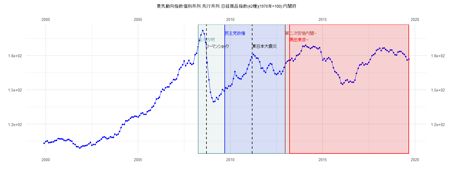
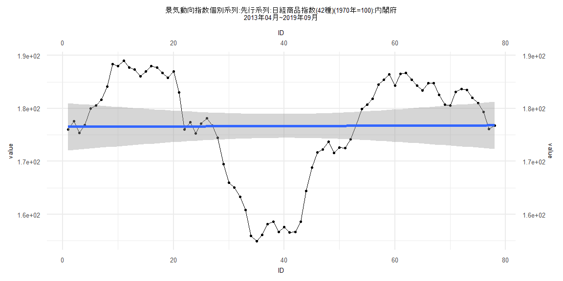
[1] "景気動向指数個別系列:先行系列:日経商品指数(42種)(1970年=100):内閣府"
         Jan     Feb     Mar     Apr     May     Jun     Jul     Aug     Sep     Oct     Nov     Dec
1999                                                                                         103.233
2000 104.701 105.219 103.769 103.919 104.311 104.572 105.646 105.929 107.467 107.015 107.155 106.778
2001 105.809 105.453 106.399 106.495 105.592 105.062 103.052 102.176 100.376 100.179  99.203 100.218
2002 100.928 100.776 101.155 101.649 102.619 103.917 101.530 102.277 102.306 104.028 104.953 105.515
2003 106.752 108.276 108.918 108.065 107.147 107.543 108.985 108.262 108.282 111.275 110.460 111.260
2004 113.551 116.821 119.731 119.795 122.794 122.926 123.543 125.081 126.178 126.294 127.013 126.864
2005 126.146 127.502 129.281 129.816 128.586 128.660 130.967 131.605 132.202 134.825 135.787 138.398
2006 142.060 142.571 143.471 148.406 150.488 149.775 151.787 152.659 152.471 155.516 156.554 158.921
2007 158.716 159.424 163.063 168.185 169.648 171.893 175.312 171.161 173.351 175.721 173.218 172.334
2008 172.938 180.651 182.145 187.634 193.277 198.164 201.914 199.048 191.535 173.662 158.652 147.854
2009 143.107 139.699 139.827 143.336 141.840 144.971 146.320 150.133 148.890 151.728 151.370 153.228
2010 153.391 154.897 159.782 165.893 162.444 160.524 159.907 159.511 161.891 163.504 164.576 168.232
2011 171.842 176.137 178.951 180.965 179.801 178.005 177.515 174.503 168.897 169.095 166.651 165.195
2012 169.100 171.372 173.106 172.526 166.968 164.232 163.420 164.424 166.262 163.824 166.279 169.679
2013 173.500 174.999 175.959 176.051 177.618 175.427 176.854 180.025 180.555 181.605 184.132 188.334
2014 187.995 189.005 187.695 187.313 186.105 187.031 187.984 187.760 186.677 185.780 186.985 183.036
2015 176.003 177.430 175.260 177.106 178.137 176.769 174.461 169.466 166.020 165.098 163.272 160.852
2016 155.948 154.942 156.095 158.194 158.665 156.704 157.572 156.636 156.713 158.586 164.413 168.833
2017 171.743 172.284 173.696 171.609 172.631 172.514 174.141 176.718 179.875 180.695 181.862 184.488
2018 185.463 186.434 184.314 186.501 186.685 185.395 184.270 183.405 184.781 184.792 182.523 180.684
2019 180.567 183.091 183.632 183.527 182.033 181.001 179.303 176.139 176.796
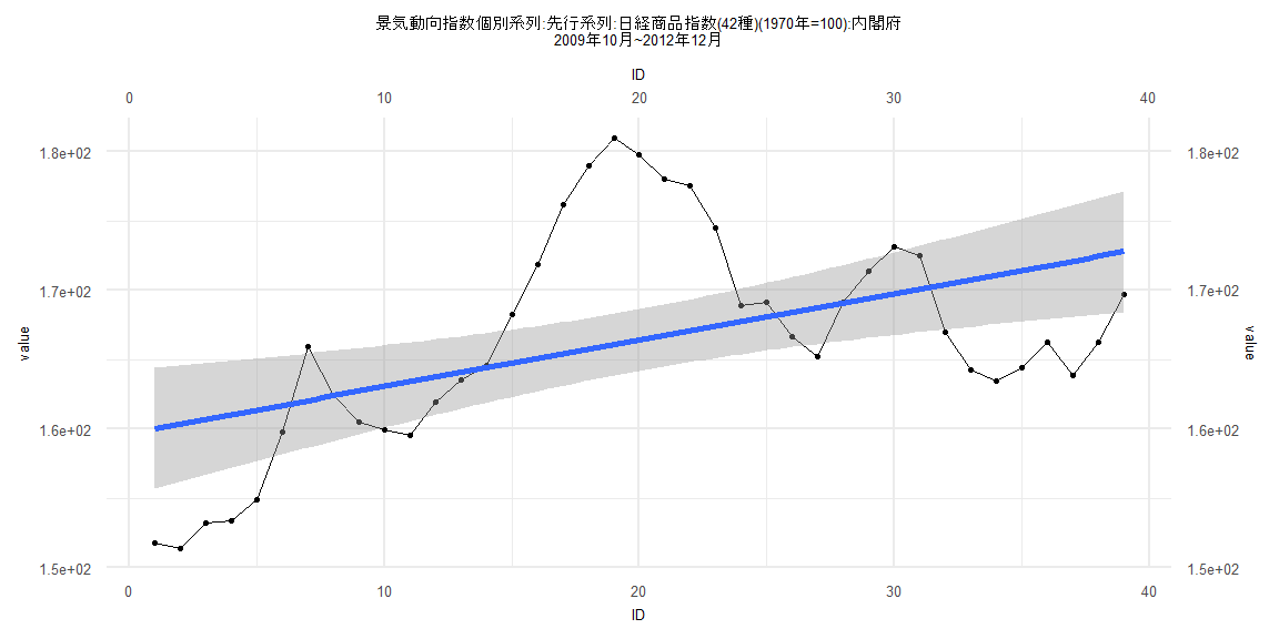
Call:
lm(formula = value ~ ID)

Residuals:
   Min     1Q Median     3Q    Max
-8.995 -5.831 -1.762  3.430 14.900

Coefficients:
             Estimate Std. Error t value             Pr(>|t|)
(Intercept) 159.69400    2.24059  71.273 < 0.0000000000000002 ***
ID            0.33533    0.09763   3.435              0.00148 **
---
Signif. codes:  0 '***' 0.001 '**' 0.01 '*' 0.05 '.' 0.1 ' ' 1

Residual standard error: 6.862 on 37 degrees of freedom
Multiple R-squared:  0.2418,    Adjusted R-squared:  0.2213
F-statistic:  11.8 on 1 and 37 DF,  p-value: 0.001478


    Two-sample Kolmogorov-Smirnov test

data:  lm_residuals and rnorm(n = length(lm_residuals), mean = 0, sd = sd(lm_residuals))
D = 0.15385, p-value = 0.7523
alternative hypothesis: two-sided


    Durbin-Watson test

data:  value ~ ID
DW = 0.16406, p-value < 0.00000000000000022
alternative hypothesis: true autocorrelation is greater than 0


    studentized Breusch-Pagan test

data:  value ~ ID
BP = 0.13421, df = 1, p-value = 0.7141


    Box-Ljung test

data:  lm_residuals
X-squared = 33.74, df = 1, p-value = 0.000000006299
Call:
lm(formula = value ~ ID)

Residuals:
    Min      1Q  Median      3Q     Max
-21.641  -4.200   1.628   7.725  12.619

Coefficients:
              Estimate Std. Error t value            Pr(>|t|)
(Intercept) 176.270835   2.201091  80.083 <0.0000000000000002 ***
ID            0.008207   0.046635   0.176               0.861
---
Signif. codes:  0 '***' 0.001 '**' 0.01 '*' 0.05 '.' 0.1 ' ' 1

Residual standard error: 9.813 on 79 degrees of freedom
Multiple R-squared:  0.0003918, Adjusted R-squared:  -0.01226
F-statistic: 0.03097 on 1 and 79 DF,  p-value: 0.8608


    Two-sample Kolmogorov-Smirnov test

data:  lm_residuals and rnorm(n = length(lm_residuals), mean = 0, sd = sd(lm_residuals))
D = 0.17284, p-value = 0.1783
alternative hypothesis: two-sided


    Durbin-Watson test

data:  value ~ ID
DW = 0.049214, p-value < 0.00000000000000022
alternative hypothesis: true autocorrelation is greater than 0


    studentized Breusch-Pagan test

data:  value ~ ID
BP = 0.2628, df = 1, p-value = 0.6082


    Box-Ljung test

data:  lm_residuals
X-squared = 79.869, df = 1, p-value < 0.00000000000000022
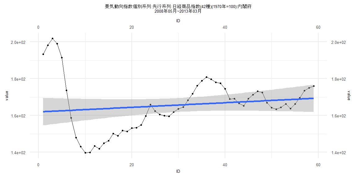
Call:
lm(formula = value ~ ID)

Residuals:
    Min      1Q  Median      3Q     Max
-23.507  -7.873  -2.196   5.787  39.581

Coefficients:
            Estimate Std. Error t value            Pr(>|t|)
(Intercept) 161.9593     3.8099  42.510 <0.0000000000000002 ***
ID            0.1247     0.1104   1.129               0.264
---
Signif. codes:  0 '***' 0.001 '**' 0.01 '*' 0.05 '.' 0.1 ' ' 1

Residual standard error: 14.45 on 57 degrees of freedom
Multiple R-squared:  0.02188,   Adjusted R-squared:  0.004716
F-statistic: 1.275 on 1 and 57 DF,  p-value: 0.2636


    Two-sample Kolmogorov-Smirnov test

data:  lm_residuals and rnorm(n = length(lm_residuals), mean = 0, sd = sd(lm_residuals))
D = 0.16949, p-value = 0.3674
alternative hypothesis: two-sided


    Durbin-Watson test

data:  value ~ ID
DW = 0.097934, p-value < 0.00000000000000022
alternative hypothesis: true autocorrelation is greater than 0


    studentized Breusch-Pagan test

data:  value ~ ID
BP = 25.526, df = 1, p-value = 0.0000004365


    Box-Ljung test

data:  lm_residuals
X-squared = 51.191, df = 1, p-value = 0.0000000000008379
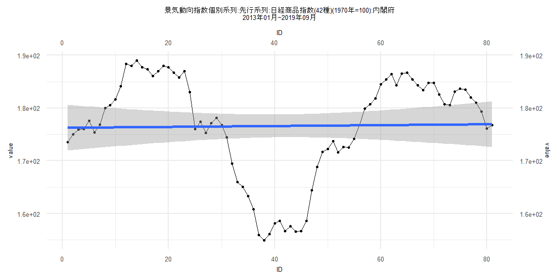
Call:
lm(formula = value ~ ID)

Residuals:
    Min      1Q  Median      3Q     Max
-21.718  -4.365   2.820   7.704  12.432

Coefficients:
              Estimate Std. Error t value            Pr(>|t|)
(Intercept) 176.532527   2.286092  77.220 <0.0000000000000002 ***
ID            0.003634   0.050281   0.072               0.943
---
Signif. codes:  0 '***' 0.001 '**' 0.01 '*' 0.05 '.' 0.1 ' ' 1

Residual standard error: 9.998 on 76 degrees of freedom
Multiple R-squared:  6.873e-05, Adjusted R-squared:  -0.01309
F-statistic: 0.005224 on 1 and 76 DF,  p-value: 0.9426


    Two-sample Kolmogorov-Smirnov test

data:  lm_residuals and rnorm(n = length(lm_residuals), mean = 0, sd = sd(lm_residuals))
D = 0.17949, p-value = 0.1624
alternative hypothesis: two-sided


    Durbin-Watson test

data:  value ~ ID
DW = 0.04887, p-value < 0.00000000000000022
alternative hypothesis: true autocorrelation is greater than 0


    studentized Breusch-Pagan test

data:  value ~ ID
BP = 0.82957, df = 1, p-value = 0.3624


    Box-Ljung test

data:  lm_residuals
X-squared = 77.125, df = 1, p-value < 0.00000000000000022