Analysis
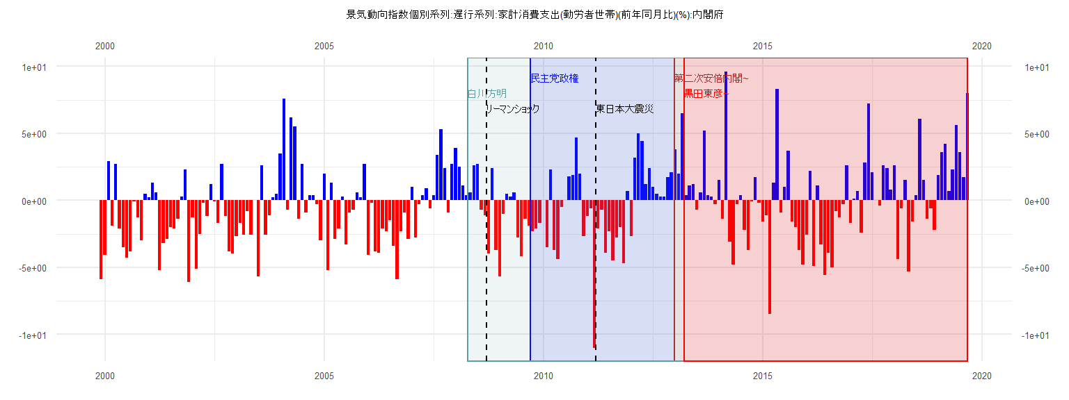
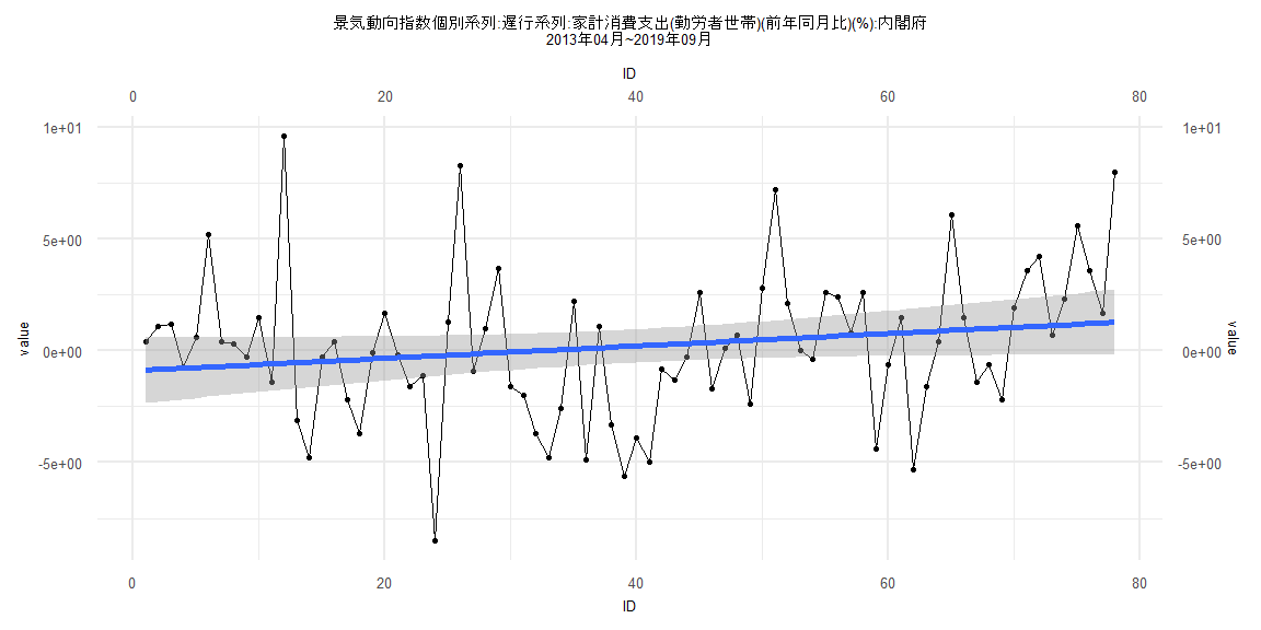
[1] "景気動向指数個別系列:遅行系列:家計消費支出(勤労者世帯)(前年同月比)(%):内閣府"
Jan Feb Mar Apr May Jun Jul Aug Sep Oct Nov Dec
1999 -5.9
2000 -4.1 2.9 -1.9 2.7 -2.1 -3.5 -4.3 -3.8 -0.1 -1.3 -3.0 0.5
2001 0.2 1.3 0.6 -5.2 -3.2 -2.9 -2.0 -2.1 -1.4 0.3 2.3 -6.1
2002 -1.3 -5.1 -2.5 -0.2 -1.2 1.2 -0.1 -1.7 2.7 -1.2 -3.8 -4.0
2003 -2.7 -1.7 -2.6 -0.8 -2.6 0.0 -5.7 2.6 -2.6 -1.1 0.2 0.5
2004 3.5 7.6 -0.7 6.2 5.5 -1.4 2.7 -0.9 0.4 0.4 -0.3 -3.0
2005 2.0 -5.2 1.3 -2.9 -2.1 0.3 -3.3 -0.9 -0.7 0.6 0.2 2.7
2006 -4.1 -0.2 -3.8 -3.9 -2.1 -2.3 -1.5 -3.4 -5.9 -2.3 -0.9 -2.9
2007 1.0 -2.8 -0.3 0.4 0.9 -0.6 0.4 3.4 5.3 2.4 -0.9 2.7
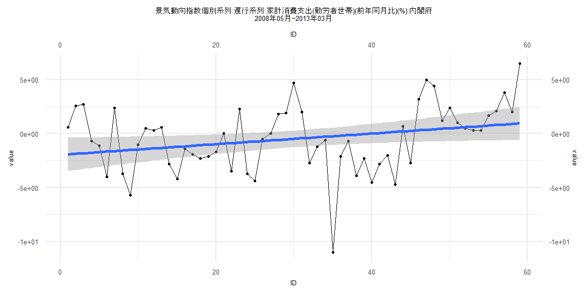
2008 3.9 2.5 1.1 0.4 0.6 2.6 2.7 -0.7 -1.1 -4.0 2.4 -3.7
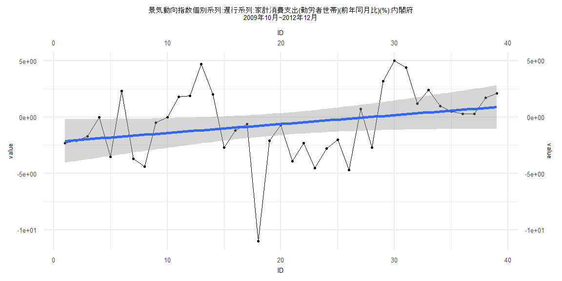
2009 -5.7 -1.0 0.5 0.3 0.6 -2.8 -4.2 -1.4 -1.9 -2.3 -2.1 -1.7
2010 0.0 -3.5 2.3 -3.7 -4.4 -0.5 0.0 1.8 1.9 4.7 2.0 -2.7
2011 -1.2 -0.6 -11.0 -2.1 -0.7 -3.9 -2.3 -4.5 -2.8 -2.0 -4.7 0.7
2012 -2.7 3.2 5.0 4.4 1.2 2.4 1.0 0.5 0.3 0.3 1.7 2.1
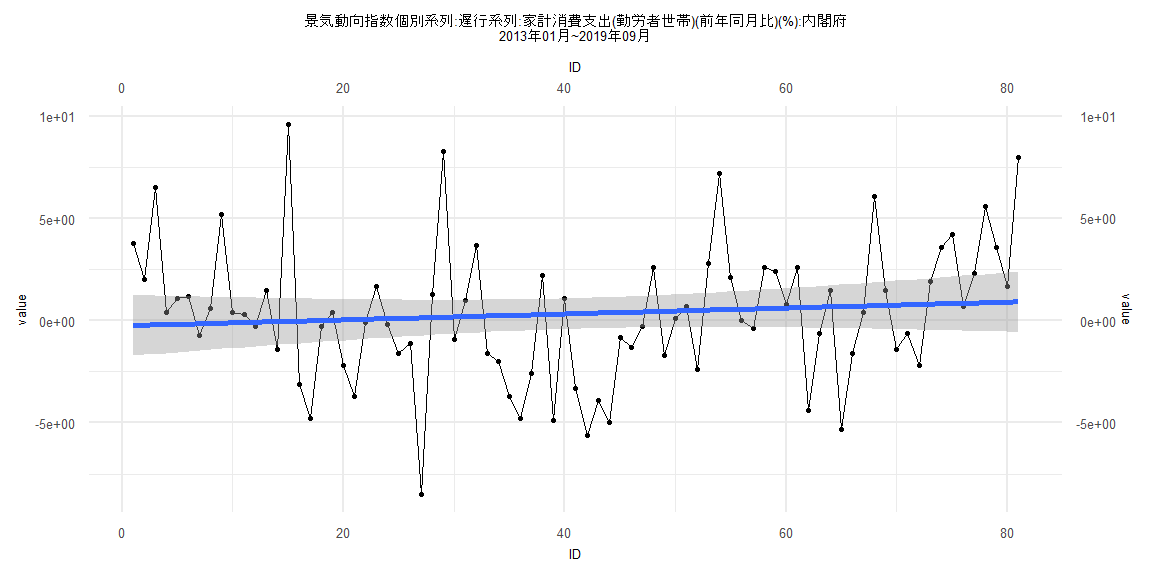
2013 3.8 2.0 6.5 0.4 1.1 1.2 -0.7 0.6 5.2 0.4 0.3 -0.3
2014 1.5 -1.4 9.6 -3.1 -4.8 -0.3 0.4 -2.2 -3.7 -0.1 1.7 -0.2
2015 -1.6 -1.1 -8.5 1.3 8.3 -0.9 1.0 3.7 -1.6 -2.0 -3.7 -4.8
2016 -2.6 2.2 -4.9 1.1 -3.3 -5.6 -3.9 -5.0 -0.8 -1.3 -0.3 2.6
2017 -1.7 0.1 0.7 -2.4 2.8 7.2 2.1 0.0 -0.4 2.6 2.4 0.8
2018 2.6 -4.4 -0.6 1.5 -5.3 -1.6 0.4 6.1 1.5 -1.4 -0.6 -2.2
2019 1.9 3.6 4.2 0.7 2.3 5.6 3.6 1.7 8.0
Call:
lm(formula = value ~ ID)

Residuals:
     Min       1Q   Median       3Q      Max
-10.2286  -1.7408  -0.0603   1.6433   5.8677

Coefficients:
            Estimate Std. Error t value Pr(>|t|)
(Intercept) -2.19825    0.98784  -2.225   0.0322 *
ID           0.07927    0.04304   1.842   0.0736 .
---
Signif. codes:  0 '***' 0.001 '**' 0.01 '*' 0.05 '.' 0.1 ' ' 1

Residual standard error: 3.025 on 37 degrees of freedom
Multiple R-squared:  0.08397,   Adjusted R-squared:  0.05921
F-statistic: 3.392 on 1 and 37 DF,  p-value: 0.07356


    Two-sample Kolmogorov-Smirnov test

data:  lm_residuals and rnorm(n = length(lm_residuals), mean = 0, sd = sd(lm_residuals))
D = 0.15385, p-value = 0.7523
alternative hypothesis: two-sided


    Durbin-Watson test

data:  value ~ ID
DW = 1.348, p-value = 0.01105
alternative hypothesis: true autocorrelation is greater than 0


    studentized Breusch-Pagan test

data:  value ~ ID
BP = 0.054556, df = 1, p-value = 0.8153


    Box-Ljung test

data:  lm_residuals
X-squared = 4.4116, df = 1, p-value = 0.03569
Call:
lm(formula = value ~ ID)

Residuals:
   Min     1Q Median     3Q    Max
-8.642 -2.162 -0.154  1.616  9.632

Coefficients:
            Estimate Std. Error t value Pr(>|t|)
(Intercept) -0.24978    0.75757  -0.330    0.742
ID           0.01452    0.01605   0.905    0.368

Residual standard error: 3.378 on 79 degrees of freedom
Multiple R-squared:  0.01026,   Adjusted R-squared:  -0.002271
F-statistic: 0.8187 on 1 and 79 DF,  p-value: 0.3683


    Two-sample Kolmogorov-Smirnov test

data:  lm_residuals and rnorm(n = length(lm_residuals), mean = 0, sd = sd(lm_residuals))
D = 0.08642, p-value = 0.9254
alternative hypothesis: two-sided


    Durbin-Watson test

data:  value ~ ID
DW = 1.5215, p-value = 0.01047
alternative hypothesis: true autocorrelation is greater than 0


    studentized Breusch-Pagan test

data:  value ~ ID
BP = 0.25085, df = 1, p-value = 0.6165


    Box-Ljung test

data:  lm_residuals
X-squared = 3.4445, df = 1, p-value = 0.06346
Call:
lm(formula = value ~ ID)

Residuals:
     Min       1Q   Median       3Q      Max
-10.7650  -2.1223   0.1784   1.9181   5.5527

Coefficients:
            Estimate Std. Error t value Pr(>|t|)
(Intercept) -1.95926    0.78625  -2.492   0.0156 *
ID           0.04926    0.02279   2.161   0.0349 *
---
Signif. codes:  0 '***' 0.001 '**' 0.01 '*' 0.05 '.' 0.1 ' ' 1

Residual standard error: 2.981 on 57 degrees of freedom
Multiple R-squared:  0.07575,   Adjusted R-squared:  0.05954
F-statistic: 4.672 on 1 and 57 DF,  p-value: 0.03488


    Two-sample Kolmogorov-Smirnov test

data:  lm_residuals and rnorm(n = length(lm_residuals), mean = 0, sd = sd(lm_residuals))
D = 0.11864, p-value = 0.8052
alternative hypothesis: two-sided


    Durbin-Watson test

data:  value ~ ID
DW = 1.2543, p-value = 0.0008801
alternative hypothesis: true autocorrelation is greater than 0


    studentized Breusch-Pagan test

data:  value ~ ID
BP = 0.11693, df = 1, p-value = 0.7324


    Box-Ljung test

data:  lm_residuals
X-squared = 7.0146, df = 1, p-value = 0.008085
Call:
lm(formula = value ~ ID)

Residuals:
    Min      1Q  Median      3Q     Max
-8.2714 -1.9185  0.1458  1.8495 10.1614

Coefficients:
            Estimate Std. Error t value Pr(>|t|)
(Intercept) -0.89417    0.75379  -1.186   0.2392
ID           0.02773    0.01658   1.673   0.0985 .
---
Signif. codes:  0 '***' 0.001 '**' 0.01 '*' 0.05 '.' 0.1 ' ' 1

Residual standard error: 3.297 on 76 degrees of freedom
Multiple R-squared:  0.03551,   Adjusted R-squared:  0.02282
F-statistic: 2.798 on 1 and 76 DF,  p-value: 0.09849


    Two-sample Kolmogorov-Smirnov test

data:  lm_residuals and rnorm(n = length(lm_residuals), mean = 0, sd = sd(lm_residuals))
D = 0.11538, p-value = 0.6802
alternative hypothesis: two-sided


    Durbin-Watson test

data:  value ~ ID
DW = 1.5863, p-value = 0.02429
alternative hypothesis: true autocorrelation is greater than 0


    studentized Breusch-Pagan test

data:  value ~ ID
BP = 0.16604, df = 1, p-value = 0.6837


    Box-Ljung test

data:  lm_residuals
X-squared = 2.5806, df = 1, p-value = 0.1082