Analysis
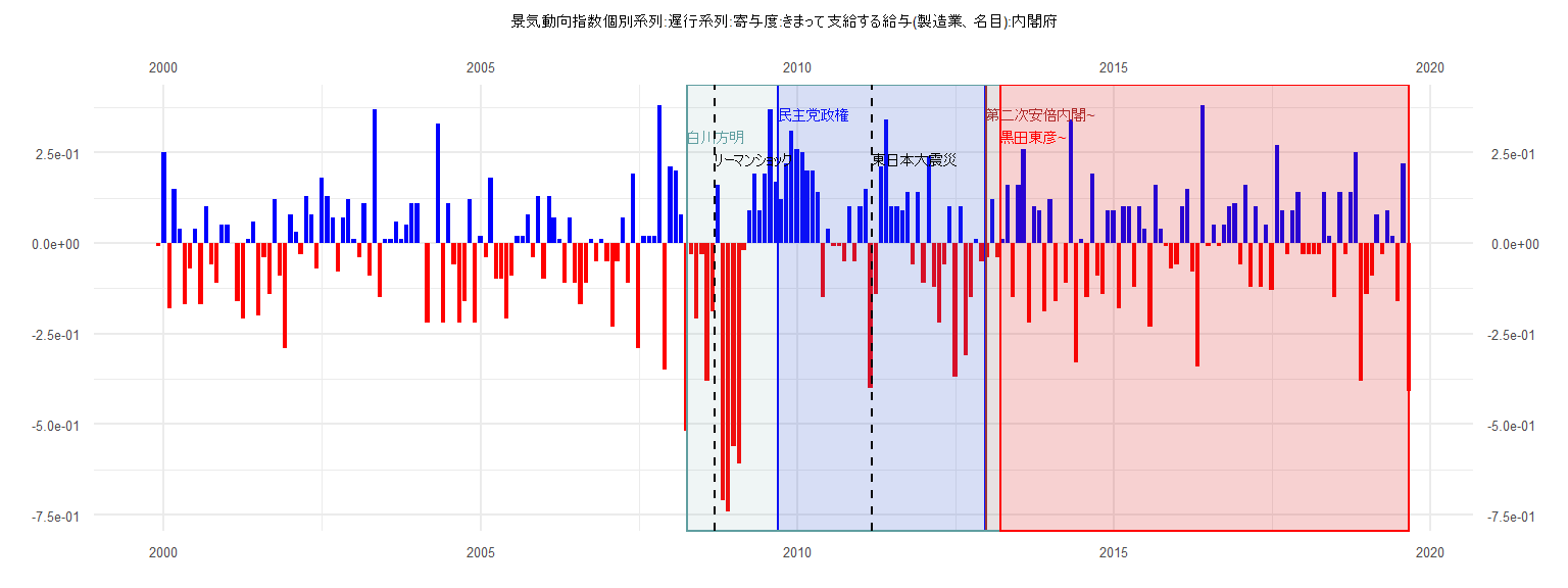
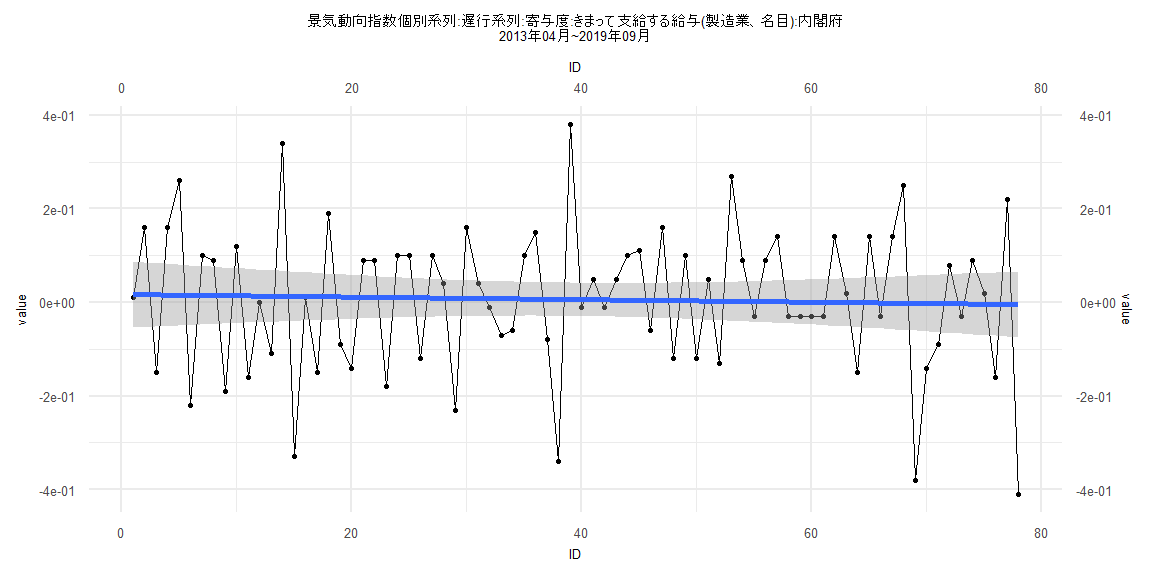
[1] "景気動向指数個別系列:遅行系列:寄与度:きまって支給する給与(製造業、名目):内閣府"
       Jan   Feb   Mar   Apr   May   Jun   Jul   Aug   Sep   Oct   Nov   Dec
1999                                                                   -0.01
2000  0.25 -0.18  0.15  0.04 -0.17 -0.07  0.04 -0.17  0.10 -0.06 -0.11  0.05
2001  0.05  0.00 -0.16 -0.21  0.01  0.06 -0.20 -0.04 -0.14  0.12 -0.09 -0.29
2002  0.08  0.03 -0.03  0.13  0.08 -0.07  0.18  0.13  0.07 -0.08  0.07  0.12
2003  0.01 -0.04  0.11 -0.09  0.37 -0.15  0.01  0.01  0.06  0.01  0.05  0.11
2004  0.11  0.00 -0.22  0.00  0.33 -0.22  0.11 -0.06 -0.22 -0.16  0.12 -0.22
2005  0.02 -0.04  0.18 -0.10 -0.10 -0.21 -0.09  0.02  0.02  0.08 -0.04  0.13
2006 -0.10  0.13  0.07  0.01 -0.11  0.07 -0.11 -0.17 -0.11  0.01 -0.05  0.01
2007 -0.05 -0.23 -0.05  0.07 -0.11  0.19 -0.29  0.02  0.02  0.02  0.38 -0.35
2008  0.21  0.20  0.08 -0.52 -0.03 -0.21 -0.03 -0.38 -0.19  0.16 -0.71 -0.74
2009 -0.56 -0.61 -0.02  0.09  0.19  0.09  0.19  0.37  0.17  0.12  0.22  0.31
2010  0.26  0.25  0.20  0.20  0.14 -0.15  0.04 -0.01 -0.01 -0.05  0.10 -0.05
2011  0.10  0.15 -0.40 -0.14  0.21  0.34  0.10  0.10  0.09  0.14 -0.06  0.14
2012 -0.11  0.24 -0.12 -0.22 -0.06  0.10 -0.37  0.10 -0.31 -0.15  0.01 -0.05
2013 -0.04  0.12 -0.04  0.01  0.16 -0.15  0.16  0.26 -0.22  0.10  0.09 -0.19
2014  0.12 -0.16  0.00 -0.11  0.34 -0.33  0.01 -0.15  0.19 -0.09 -0.14  0.09
2015  0.09 -0.18  0.10  0.10 -0.12  0.10  0.04 -0.23  0.16  0.04 -0.01 -0.07
2016 -0.06  0.10  0.15 -0.08 -0.34  0.38 -0.01  0.05 -0.01  0.05  0.10  0.11
2017 -0.06  0.16 -0.12  0.10 -0.12  0.05 -0.13  0.27  0.09 -0.03  0.09  0.14
2018 -0.03 -0.03 -0.03 -0.03  0.14  0.02 -0.15  0.14 -0.03  0.14  0.25 -0.38
2019 -0.14 -0.09  0.08 -0.03  0.09  0.02 -0.16  0.22 -0.41
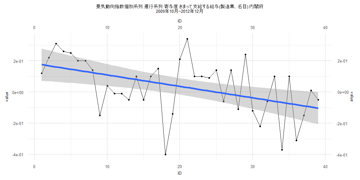
Call:
lm(formula = value ~ ID)

Residuals:
    Min      1Q  Median      3Q     Max
-0.4506 -0.0959  0.0348  0.1051  0.3114

Coefficients:
             Estimate Std. Error t value Pr(>|t|)
(Intercept)  0.182416   0.052852   3.451  0.00141 **
ID          -0.007326   0.002303  -3.181  0.00297 **
---
Signif. codes:  0 '***' 0.001 '**' 0.01 '*' 0.05 '.' 0.1 ' ' 1

Residual standard error: 0.1619 on 37 degrees of freedom
Multiple R-squared:  0.2148,    Adjusted R-squared:  0.1935
F-statistic: 10.12 on 1 and 37 DF,  p-value: 0.002967


    Two-sample Kolmogorov-Smirnov test

data:  lm_residuals and rnorm(n = length(lm_residuals), mean = 0, sd = sd(lm_residuals))
D = 0.20513, p-value = 0.3888
alternative hypothesis: two-sided


    Durbin-Watson test

data:  value ~ ID
DW = 1.9711, p-value = 0.3961
alternative hypothesis: true autocorrelation is greater than 0


    studentized Breusch-Pagan test

data:  value ~ ID
BP = 0.64756, df = 1, p-value = 0.421


    Box-Ljung test

data:  lm_residuals
X-squared = 0.0054741, df = 1, p-value = 0.941
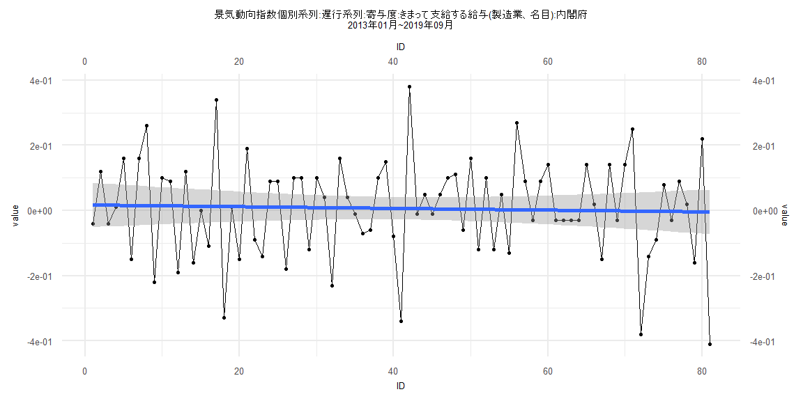
Call:
lm(formula = value ~ ID)

Residuals:
     Min       1Q   Median       3Q      Max
-0.40594 -0.10140 -0.00218  0.09515  0.37384

Coefficients:
              Estimate Std. Error t value Pr(>|t|)
(Intercept)  0.0171605  0.0348157   0.493    0.623
ID          -0.0002620  0.0007376  -0.355    0.723

Residual standard error: 0.1552 on 79 degrees of freedom
Multiple R-squared:  0.001594,  Adjusted R-squared:  -0.01104
F-statistic: 0.1261 on 1 and 79 DF,  p-value: 0.7234


    Two-sample Kolmogorov-Smirnov test

data:  lm_residuals and rnorm(n = length(lm_residuals), mean = 0, sd = sd(lm_residuals))
D = 0.074074, p-value = 0.9806
alternative hypothesis: two-sided


    Durbin-Watson test

data:  value ~ ID
DW = 2.7094, p-value = 0.9993
alternative hypothesis: true autocorrelation is greater than 0


    studentized Breusch-Pagan test

data:  value ~ ID
BP = 0.21466, df = 1, p-value = 0.6431


    Box-Ljung test

data:  lm_residuals
X-squared = 13.368, df = 1, p-value = 0.000256
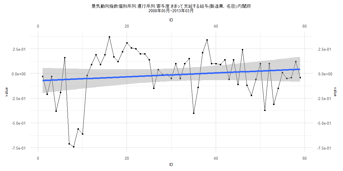
Call:
lm(formula = value ~ ID)

Residuals:
     Min       1Q   Median       3Q      Max
-0.68371 -0.12699  0.05909  0.15986  0.41063

Coefficients:
             Estimate Std. Error t value Pr(>|t|)
(Intercept) -0.071958   0.065074  -1.106    0.273
ID           0.001958   0.001886   1.038    0.304

Residual standard error: 0.2468 on 57 degrees of freedom
Multiple R-squared:  0.01855,   Adjusted R-squared:  0.00133
F-statistic: 1.077 on 1 and 57 DF,  p-value: 0.3037


    Two-sample Kolmogorov-Smirnov test

data:  lm_residuals and rnorm(n = length(lm_residuals), mean = 0, sd = sd(lm_residuals))
D = 0.15254, p-value = 0.5021
alternative hypothesis: two-sided


    Durbin-Watson test

data:  value ~ ID
DW = 1.0277, p-value = 0.0000164
alternative hypothesis: true autocorrelation is greater than 0


    studentized Breusch-Pagan test

data:  value ~ ID
BP = 6.9927, df = 1, p-value = 0.008184


    Box-Ljung test

data:  lm_residuals
X-squared = 14.592, df = 1, p-value = 0.0001335
Call:
lm(formula = value ~ ID)

Residuals:
     Min       1Q   Median       3Q      Max
-0.40568 -0.11791  0.00885  0.09461  0.37371

Coefficients:
              Estimate Std. Error t value Pr(>|t|)
(Intercept)  0.0169031  0.0360224   0.469    0.640
ID          -0.0002721  0.0007923  -0.343    0.732

Residual standard error: 0.1575 on 76 degrees of freedom
Multiple R-squared:  0.00155,   Adjusted R-squared:  -0.01159
F-statistic: 0.118 on 1 and 76 DF,  p-value: 0.7322


    Two-sample Kolmogorov-Smirnov test

data:  lm_residuals and rnorm(n = length(lm_residuals), mean = 0, sd = sd(lm_residuals))
D = 0.16667, p-value = 0.2297
alternative hypothesis: two-sided


    Durbin-Watson test

data:  value ~ ID
DW = 2.7055, p-value = 0.9991
alternative hypothesis: true autocorrelation is greater than 0


    studentized Breusch-Pagan test

data:  value ~ ID
BP = 0.030659, df = 1, p-value = 0.861


    Box-Ljung test

data:  lm_residuals
X-squared = 12.732, df = 1, p-value = 0.0003595