Analysis
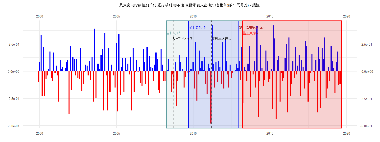
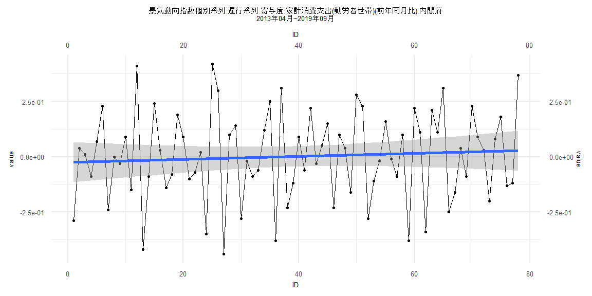
[1] "景気動向指数個別系列:遅行系列:寄与度:家計消費支出(勤労者世帯)(前年同月比):内閣府"
       Jan   Feb   Mar   Apr   May   Jun   Jul   Aug   Sep   Oct   Nov   Dec
1999                                                                   -0.10
2000  0.08  0.33 -0.23  0.22 -0.23 -0.07 -0.04  0.02  0.18 -0.06 -0.09  0.17
2001 -0.02  0.05 -0.04 -0.28  0.10  0.02  0.04  0.00  0.03  0.08  0.10 -0.39
2002  0.23 -0.17  0.13  0.11 -0.04  0.11 -0.06 -0.07  0.21 -0.18 -0.12 -0.01
2003  0.06  0.05 -0.04  0.09 -0.08  0.13 -0.28  0.39 -0.25  0.07  0.07  0.02
2004  0.15  0.20 -0.36  0.35 -0.04 -0.36  0.21 -0.19  0.06  0.00 -0.04 -0.15
2005  0.26 -0.37  0.34 -0.22  0.04  0.12 -0.19  0.12  0.01  0.07 -0.03  0.13
2006 -0.36  0.21 -0.19 -0.01  0.10 -0.01  0.04 -0.11 -0.14  0.20  0.08 -0.12
2007  0.22 -0.22  0.14  0.04  0.03 -0.09  0.06  0.17  0.11 -0.17 -0.20  0.20
2008  0.06 -0.09 -0.09 -0.04  0.01  0.11  0.00 -0.19 -0.03 -0.16  0.08 -0.32
2009 -0.09  0.15  0.08  0.00  0.02 -0.15 -0.05  0.13 -0.02 -0.01  0.02  0.02
2010  0.08 -0.16  0.27 -0.27 -0.03  0.19  0.03  0.09  0.01  0.13 -0.12 -0.21
2011  0.07  0.03 -0.48  0.42  0.07 -0.15  0.08 -0.10  0.09  0.04 -0.12  0.27
2012 -0.16  0.29  0.09 -0.03 -0.15  0.06 -0.06 -0.02  0.00  0.01  0.07  0.03
2013  0.09 -0.08  0.22 -0.29  0.04  0.01 -0.09  0.07  0.23 -0.24  0.00 -0.03
2014  0.09 -0.15  0.41 -0.42 -0.09  0.24  0.03 -0.14 -0.08  0.19  0.09 -0.10
2015 -0.07  0.02 -0.35  0.42  0.30 -0.44  0.10  0.14 -0.28 -0.02 -0.09 -0.06
2016  0.12  0.25 -0.38  0.31 -0.23 -0.12  0.09 -0.06  0.22 -0.03  0.05  0.15
2017 -0.23  0.10  0.04 -0.16  0.28  0.23 -0.28 -0.11 -0.02  0.16 -0.01 -0.09
2018  0.10 -0.38  0.22  0.11 -0.34  0.21  0.11  0.31 -0.25 -0.16  0.04 -0.09
2019  0.23  0.09  0.03 -0.20  0.08  0.18 -0.13 -0.12  0.37
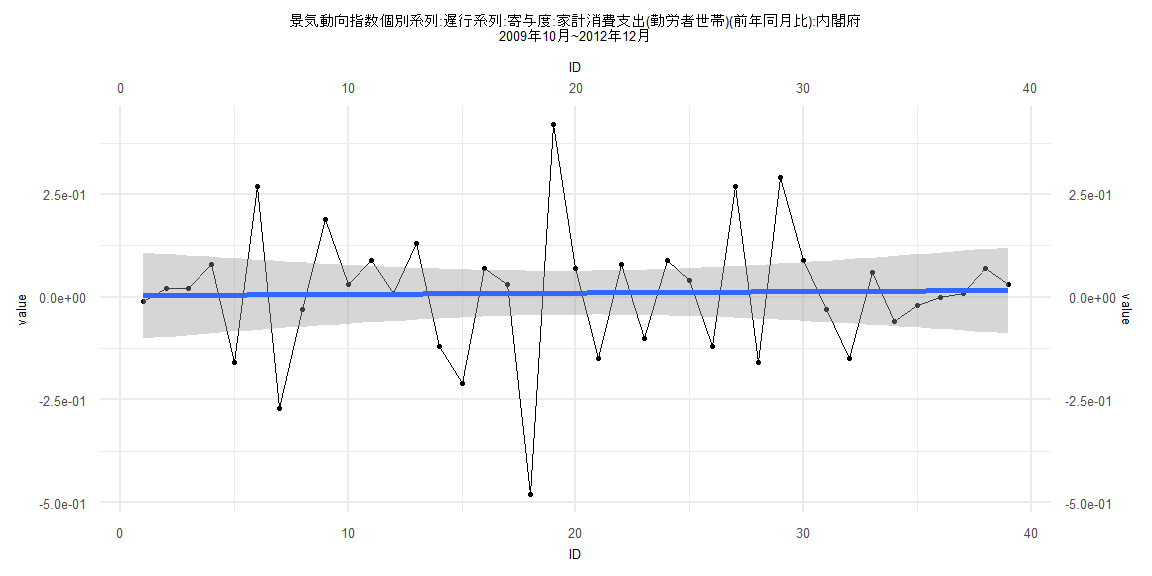
Call:
lm(formula = value ~ ID)

Residuals:
     Min       1Q   Median       3Q      Max
-0.48934 -0.09280  0.01561  0.07231  0.41033

Coefficients:
            Estimate Std. Error t value Pr(>|t|)
(Intercept) 0.003401   0.053782   0.063    0.950
ID          0.000330   0.002344   0.141    0.889

Residual standard error: 0.1647 on 37 degrees of freedom
Multiple R-squared:  0.0005355, Adjusted R-squared:  -0.02648
F-statistic: 0.01982 on 1 and 37 DF,  p-value: 0.8888


    Two-sample Kolmogorov-Smirnov test

data:  lm_residuals and rnorm(n = length(lm_residuals), mean = 0, sd = sd(lm_residuals))
D = 0.20513, p-value = 0.3888
alternative hypothesis: two-sided


    Durbin-Watson test

data:  value ~ ID
DW = 2.8986, p-value = 0.9976
alternative hypothesis: true autocorrelation is greater than 0


    studentized Breusch-Pagan test

data:  value ~ ID
BP = 0.30657, df = 1, p-value = 0.5798


    Box-Ljung test

data:  lm_residuals
X-squared = 8.5013, df = 1, p-value = 0.003549
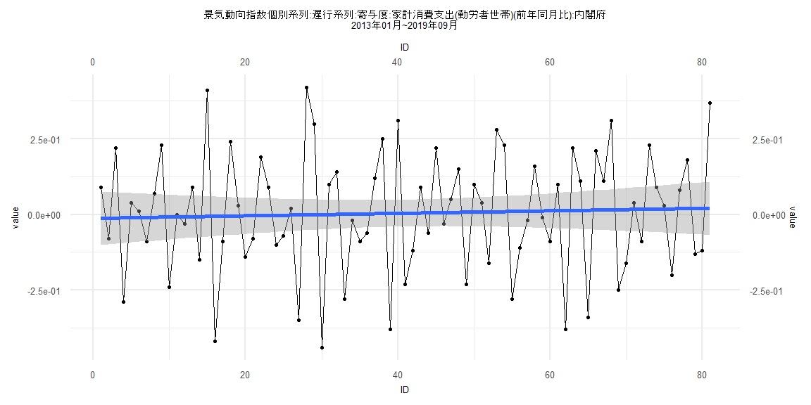
Call:
lm(formula = value ~ ID)

Residuals:
     Min       1Q   Median       3Q      Max
-0.43989 -0.12486  0.02005  0.13928  0.42094

Coefficients:
              Estimate Std. Error t value Pr(>|t|)
(Intercept) -0.0125370  0.0451422  -0.278    0.782
ID           0.0004142  0.0009564   0.433    0.666

Residual standard error: 0.2013 on 79 degrees of freedom
Multiple R-squared:  0.002368,  Adjusted R-squared:  -0.01026
F-statistic: 0.1875 on 1 and 79 DF,  p-value: 0.6662


    Two-sample Kolmogorov-Smirnov test

data:  lm_residuals and rnorm(n = length(lm_residuals), mean = 0, sd = sd(lm_residuals))
D = 0.08642, p-value = 0.9254
alternative hypothesis: two-sided


    Durbin-Watson test

data:  value ~ ID
DW = 2.7012, p-value = 0.9992
alternative hypothesis: true autocorrelation is greater than 0


    studentized Breusch-Pagan test

data:  value ~ ID
BP = 0.014097, df = 1, p-value = 0.9055


    Box-Ljung test

data:  lm_residuals
X-squared = 11.584, df = 1, p-value = 0.000665
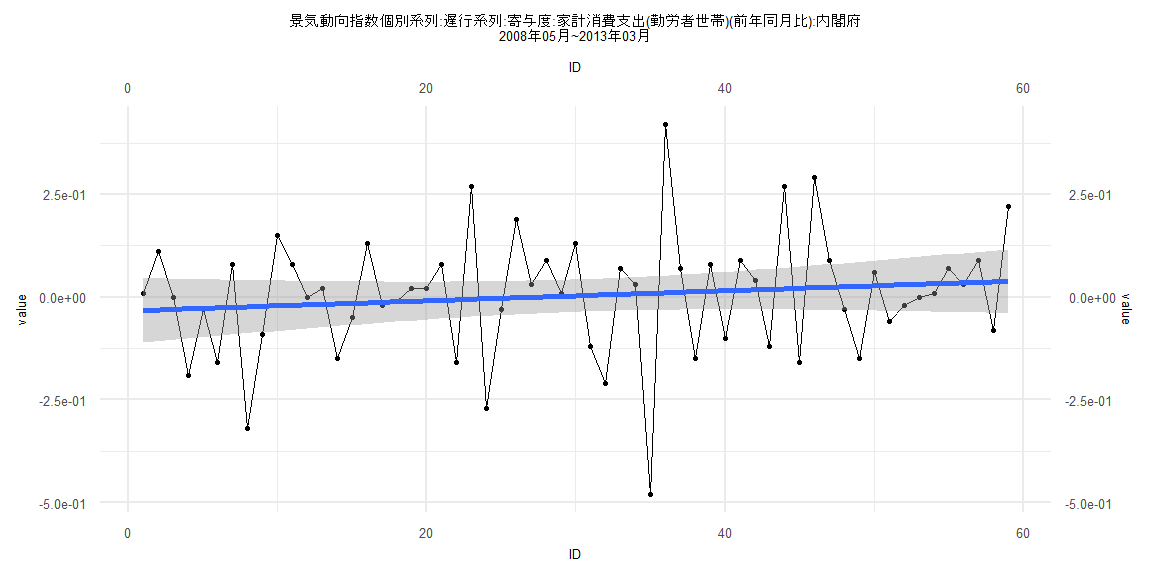
Call:
lm(formula = value ~ ID)

Residuals:
     Min       1Q   Median       3Q      Max
-0.48933 -0.10216  0.02189  0.06967  0.40945

Coefficients:
             Estimate Std. Error t value Pr(>|t|)
(Intercept) -0.033442   0.039955  -0.837    0.406
ID           0.001222   0.001158   1.055    0.296

Residual standard error: 0.1515 on 57 degrees of freedom
Multiple R-squared:  0.01916,   Adjusted R-squared:  0.00195
F-statistic: 1.113 on 1 and 57 DF,  p-value: 0.2958


    Two-sample Kolmogorov-Smirnov test

data:  lm_residuals and rnorm(n = length(lm_residuals), mean = 0, sd = sd(lm_residuals))
D = 0.15254, p-value = 0.5021
alternative hypothesis: two-sided


    Durbin-Watson test

data:  value ~ ID
DW = 2.7258, p-value = 0.9971
alternative hypothesis: true autocorrelation is greater than 0


    studentized Breusch-Pagan test

data:  value ~ ID
BP = 0.050214, df = 1, p-value = 0.8227


    Box-Ljung test

data:  lm_residuals
X-squared = 8.7798, df = 1, p-value = 0.003046
Call:
lm(formula = value ~ ID)

Residuals:
     Min       1Q   Median       3Q      Max
-0.43314 -0.12506  0.01936  0.13896  0.42823

Coefficients:
              Estimate Std. Error t value Pr(>|t|)
(Intercept) -0.0252914  0.0463848  -0.545    0.587
ID           0.0006825  0.0010202   0.669    0.506

Residual standard error: 0.2029 on 76 degrees of freedom
Multiple R-squared:  0.005854,  Adjusted R-squared:  -0.007227
F-statistic: 0.4475 on 1 and 76 DF,  p-value: 0.5055


    Two-sample Kolmogorov-Smirnov test

data:  lm_residuals and rnorm(n = length(lm_residuals), mean = 0, sd = sd(lm_residuals))
D = 0.10256, p-value = 0.81
alternative hypothesis: two-sided


    Durbin-Watson test

data:  value ~ ID
DW = 2.6423, p-value = 0.9975
alternative hypothesis: true autocorrelation is greater than 0


    studentized Breusch-Pagan test

data:  value ~ ID
BP = 0.1109, df = 1, p-value = 0.7391


    Box-Ljung test

data:  lm_residuals
X-squared = 9.9915, df = 1, p-value = 0.001573