Analysis
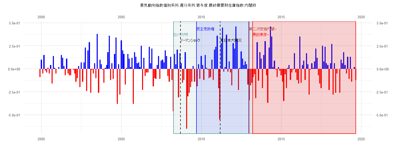
[1] "景気動向指数個別系列:遅行系列:寄与度:最終需要財在庫指数:内閣府"
       Jan   Feb   Mar   Apr   May   Jun   Jul   Aug   Sep   Oct   Nov   Dec
1999                                                                   -0.09
2000  0.10 -0.05  0.15 -0.02 -0.04  0.01 -0.05  0.04 -0.16  0.14  0.01 -0.05
2001  0.00  0.02  0.00  0.15  0.12  0.03 -0.07  0.11 -0.05 -0.07 -0.07  0.00
2002 -0.01 -0.05 -0.14 -0.10  0.03 -0.20  0.07 -0.14  0.07  0.23 -0.24  0.20
2003  0.29 -0.26 -0.01 -0.05  0.06 -0.10  0.38 -0.26  0.10  0.05 -0.01 -0.15
2004  0.01  0.04  0.18  0.36 -0.12  0.06 -0.11  0.16  0.34 -0.38  0.05 -0.28
2005  0.31  0.20  0.16 -0.17  0.01  0.16  0.11  0.02  0.12 -0.38  0.18  0.13
2006  0.06  0.07  0.02  0.25 -0.23  0.12 -0.08 -0.04 -0.04  0.24  0.06  0.22
2007 -0.19 -0.10 -0.11  0.04  0.14 -0.11  0.09  0.10  0.07  0.20  0.14 -0.08
2008 -0.14  0.13 -0.12 -0.46  0.16  0.05  0.21 -0.31  0.17  0.06 -0.15 -0.12
2009  0.18 -0.65 -0.30 -0.26 -0.20 -0.14  0.03 -0.14  0.00 -0.19  0.05 -0.11
2010  0.14  0.04 -0.12  0.15  0.01 -0.01 -0.10 -0.09  0.10 -0.12  0.21  0.24
2011  0.36 -0.21 -0.55  0.28  0.45 -0.03  0.02  0.37 -0.03  0.08 -0.04 -0.18
2012  0.28  0.22  0.46  0.32 -0.23  0.01  0.19  0.11  0.04  0.08  0.05 -0.17
2013 -0.34 -0.18 -0.15 -0.09 -0.06 -0.32  0.29 -0.13  0.18  0.11 -0.21  0.15
2014  0.30 -0.07 -0.37  0.23  0.46  0.35  0.02  0.09 -0.01 -0.09  0.02 -0.02
2015 -0.07 -0.14 -0.35 -0.06 -0.21  0.01  0.04 -0.12 -0.04 -0.01  0.17 -0.04
2016 -0.12 -0.16  0.35 -0.15  0.04  0.09 -0.12  0.17  0.05 -0.28 -0.01  0.06
2017  0.01  0.08  0.22  0.12 -0.07 -0.16 -0.21  0.25  0.08  0.24  0.06  0.04
2018 -0.23  0.06  0.27 -0.28  0.06 -0.26 -0.05  0.00 -0.26  0.10  0.06  0.18
2019  0.04 -0.05  0.13 -0.11  0.13 -0.14  0.00  0.02 -0.12
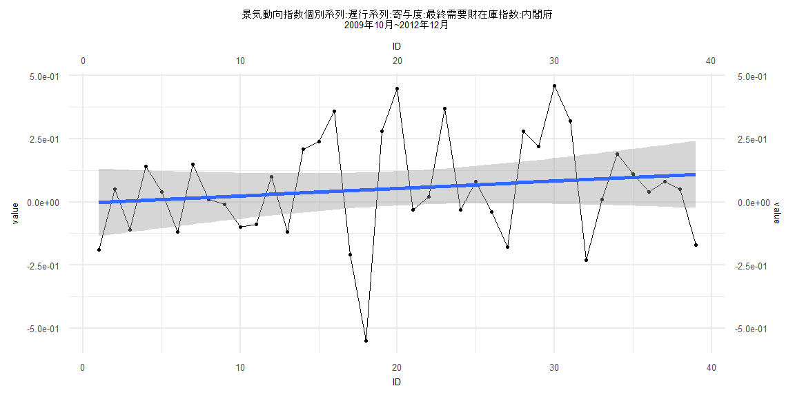
Call:
lm(formula = value ~ ID)

Residuals:
     Min       1Q   Median       3Q      Max
-0.59748 -0.11531 -0.02306  0.13752  0.39667

Coefficients:
             Estimate Std. Error t value Pr(>|t|)
(Intercept) -0.005169   0.068280  -0.076    0.940
ID           0.002925   0.002975   0.983    0.332

Residual standard error: 0.2091 on 37 degrees of freedom
Multiple R-squared:  0.02546,   Adjusted R-squared:  -0.0008806
F-statistic: 0.9666 on 1 and 37 DF,  p-value: 0.3319


    Two-sample Kolmogorov-Smirnov test

data:  lm_residuals and rnorm(n = length(lm_residuals), mean = 0, sd = sd(lm_residuals))
D = 0.17949, p-value = 0.5622
alternative hypothesis: two-sided


    Durbin-Watson test

data:  value ~ ID
DW = 1.8283, p-value = 0.2374
alternative hypothesis: true autocorrelation is greater than 0


    studentized Breusch-Pagan test

data:  value ~ ID
BP = 0.29506, df = 1, p-value = 0.587


    Box-Ljung test

data:  lm_residuals
X-squared = 0.10906, df = 1, p-value = 0.7412
Call:
lm(formula = value ~ ID)

Residuals:
     Min       1Q   Median       3Q      Max
-0.35322 -0.11723 -0.00070  0.09615  0.47599

Coefficients:
              Estimate Std. Error t value Pr(>|t|)
(Intercept) -0.0226821  0.0394460  -0.575    0.567
ID           0.0003936  0.0008358   0.471    0.639

Residual standard error: 0.1759 on 79 degrees of freedom
Multiple R-squared:  0.0028,    Adjusted R-squared:  -0.009823
F-statistic: 0.2218 on 1 and 79 DF,  p-value: 0.6389


    Two-sample Kolmogorov-Smirnov test

data:  lm_residuals and rnorm(n = length(lm_residuals), mean = 0, sd = sd(lm_residuals))
D = 0.1358, p-value = 0.4462
alternative hypothesis: two-sided


    Durbin-Watson test

data:  value ~ ID
DW = 1.9043, p-value = 0.2919
alternative hypothesis: true autocorrelation is greater than 0


    studentized Breusch-Pagan test

data:  value ~ ID
BP = 4.7339, df = 1, p-value = 0.02957


    Box-Ljung test

data:  lm_residuals
X-squared = 0.047573, df = 1, p-value = 0.8273
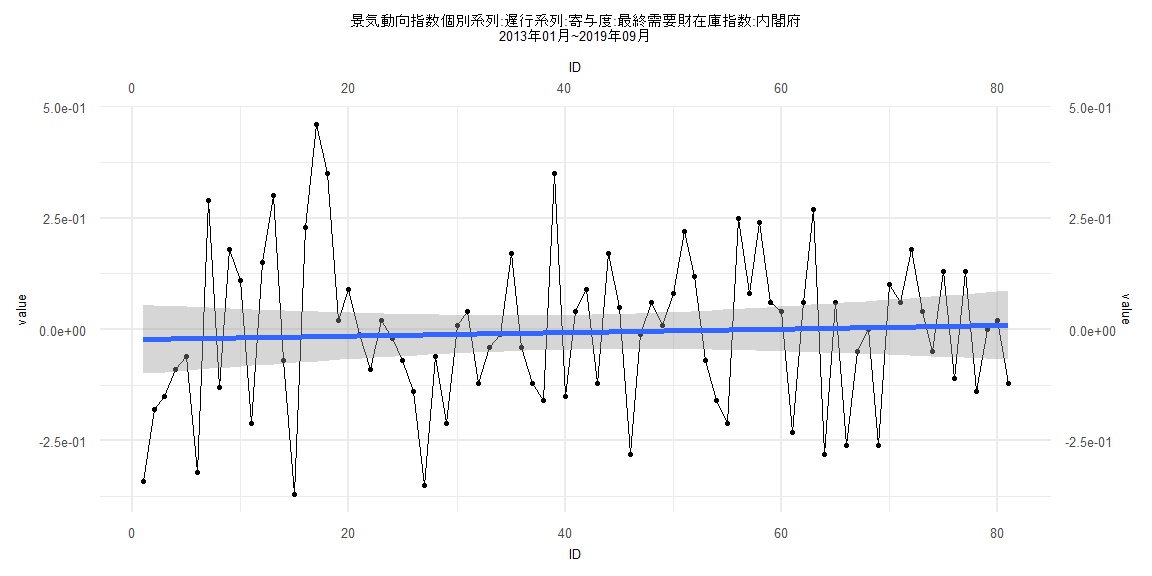
Call:
lm(formula = value ~ ID)

Residuals:
     Min       1Q   Median       3Q      Max
-0.61033 -0.11611  0.00041  0.15988  0.43611

Coefficients:
             Estimate Std. Error t value Pr(>|t|)
(Intercept) -0.059509   0.058500  -1.017    0.313
ID           0.001984   0.001696   1.170    0.247

Residual standard error: 0.2218 on 57 degrees of freedom
Multiple R-squared:  0.02344,   Adjusted R-squared:  0.006309
F-statistic: 1.368 on 1 and 57 DF,  p-value: 0.247


    Two-sample Kolmogorov-Smirnov test

data:  lm_residuals and rnorm(n = length(lm_residuals), mean = 0, sd = sd(lm_residuals))
D = 0.15254, p-value = 0.5021
alternative hypothesis: two-sided


    Durbin-Watson test

data:  value ~ ID
DW = 1.6523, p-value = 0.06807
alternative hypothesis: true autocorrelation is greater than 0


    studentized Breusch-Pagan test

data:  value ~ ID
BP = 0.075547, df = 1, p-value = 0.7834


    Box-Ljung test

data:  lm_residuals
X-squared = 1.5439, df = 1, p-value = 0.214
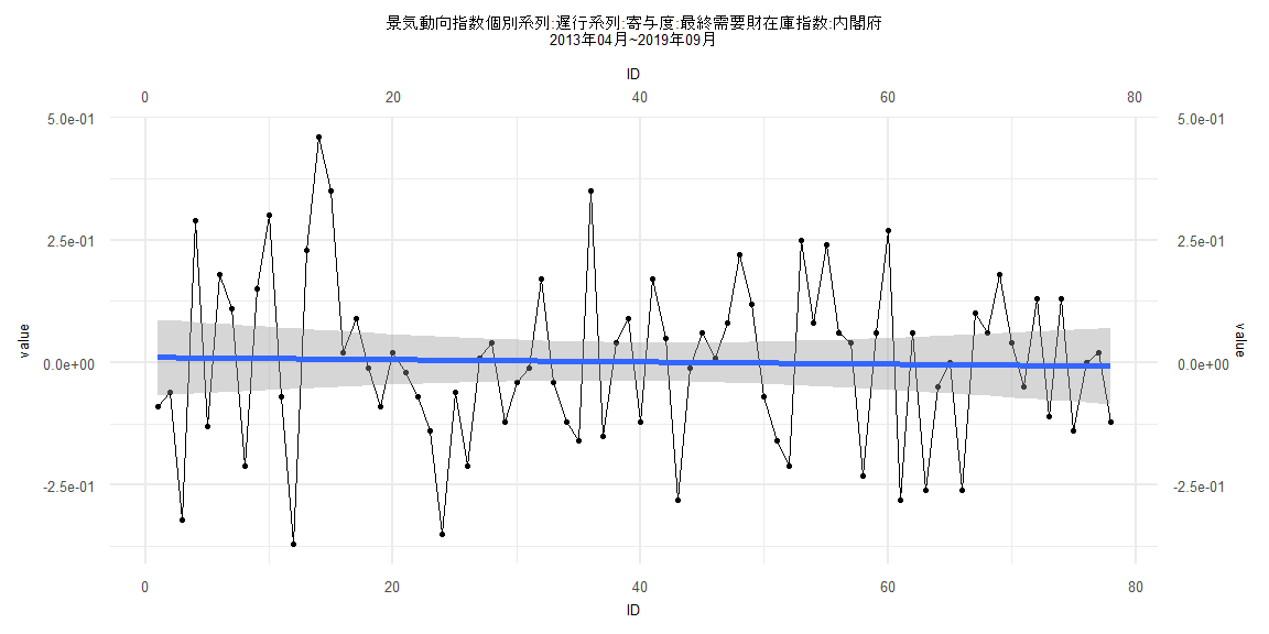
Call:
lm(formula = value ~ ID)

Residuals:
     Min       1Q   Median       3Q      Max
-0.37812 -0.11949  0.00597  0.09757  0.45234

Coefficients:
              Estimate Std. Error t value Pr(>|t|)
(Intercept)  0.0108858  0.0396108   0.275    0.784
ID          -0.0002301  0.0008712  -0.264    0.792

Residual standard error: 0.1732 on 76 degrees of freedom
Multiple R-squared:  0.0009174, Adjusted R-squared:  -0.01223
F-statistic: 0.06979 on 1 and 76 DF,  p-value: 0.7924


    Two-sample Kolmogorov-Smirnov test

data:  lm_residuals and rnorm(n = length(lm_residuals), mean = 0, sd = sd(lm_residuals))
D = 0.10256, p-value = 0.81
alternative hypothesis: two-sided


    Durbin-Watson test

data:  value ~ ID
DW = 2.0268, p-value = 0.5006
alternative hypothesis: true autocorrelation is greater than 0


    studentized Breusch-Pagan test

data:  value ~ ID
BP = 4.2806, df = 1, p-value = 0.03855


    Box-Ljung test

data:  lm_residuals
X-squared = 0.027523, df = 1, p-value = 0.8682