Analysis
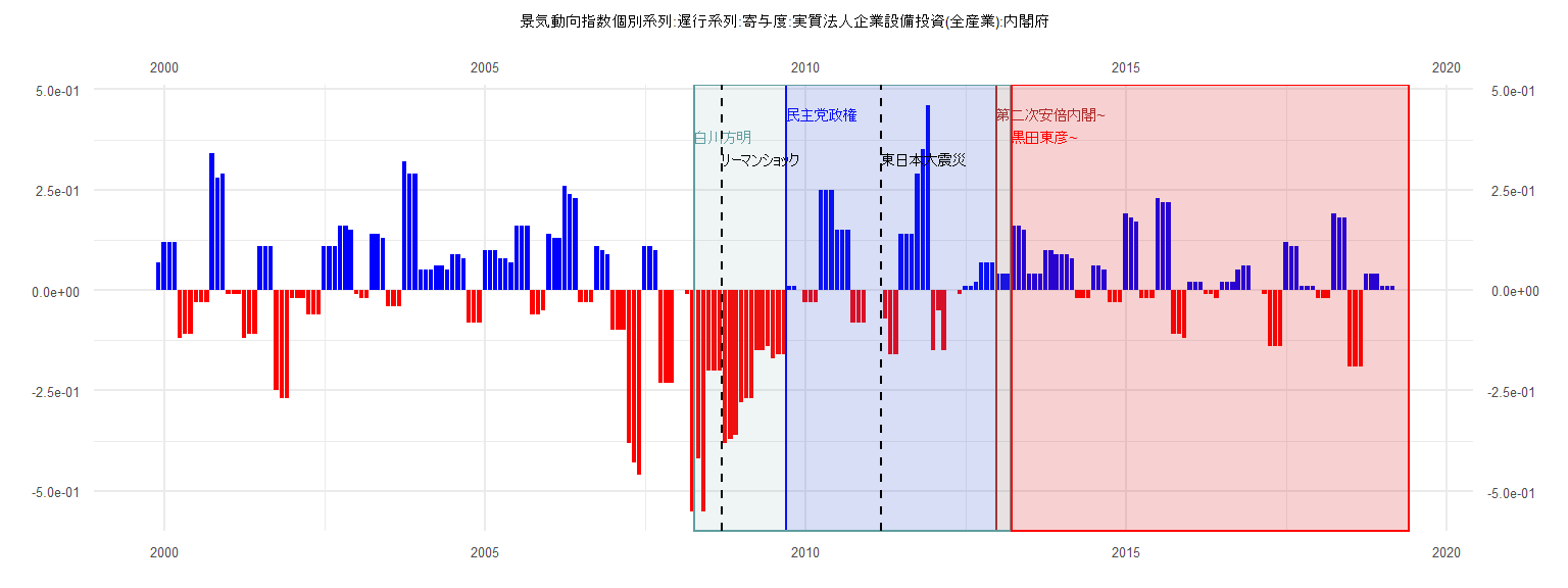
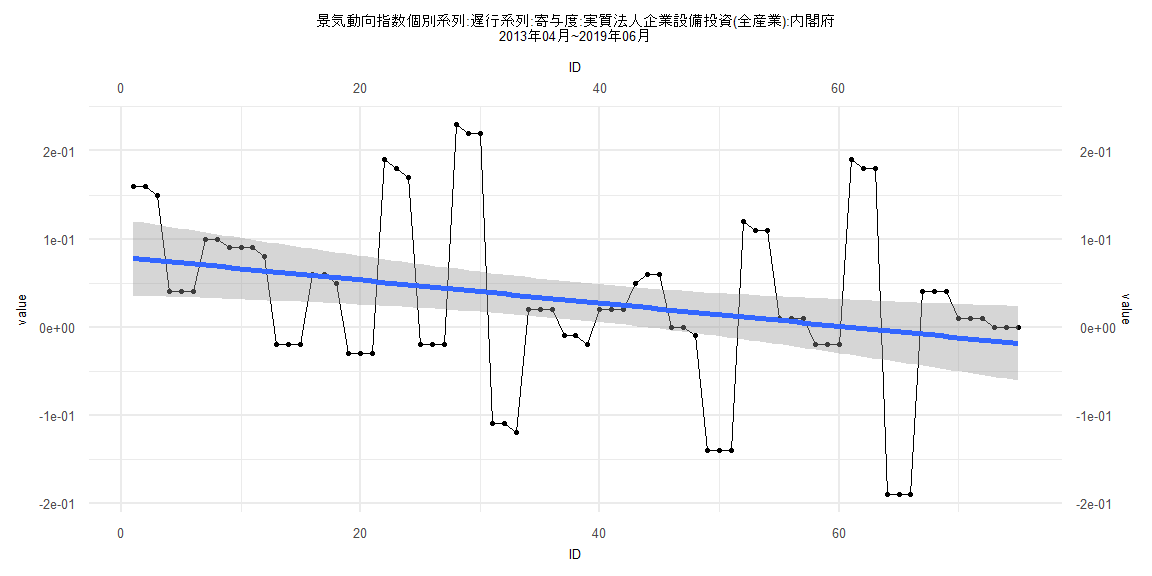
[1] "景気動向指数個別系列:遅行系列:寄与度:実質法人企業設備投資(全産業):内閣府"
       Jan   Feb   Mar   Apr   May   Jun   Jul   Aug   Sep   Oct   Nov   Dec
1999                                                                    0.07
2000  0.12  0.12  0.12 -0.12 -0.11 -0.11 -0.03 -0.03 -0.03  0.34  0.28  0.29
2001 -0.01 -0.01 -0.01 -0.12 -0.11 -0.11  0.11  0.11  0.11 -0.25 -0.27 -0.27
2002 -0.02 -0.02 -0.02 -0.06 -0.06 -0.06  0.11  0.11  0.11  0.16  0.16  0.15
2003 -0.01 -0.02 -0.02  0.14  0.14  0.13 -0.04 -0.04 -0.04  0.32  0.29  0.29
2004  0.05  0.05  0.05  0.06  0.06  0.05  0.09  0.09  0.08 -0.08 -0.08 -0.08
2005  0.10  0.10  0.10  0.08  0.08  0.07  0.16  0.16  0.16 -0.06 -0.06 -0.05
2006  0.14  0.13  0.13  0.26  0.24  0.23 -0.03 -0.03 -0.03  0.11  0.10  0.09
2007 -0.10 -0.10 -0.10 -0.38 -0.43 -0.46  0.11  0.11  0.10 -0.23 -0.23 -0.23
2008  0.00  0.00 -0.01 -0.55 -0.42 -0.55 -0.20 -0.20 -0.20 -0.38 -0.37 -0.36
2009 -0.28 -0.27 -0.27 -0.15 -0.15 -0.14 -0.17 -0.16 -0.16  0.01  0.01  0.00
2010 -0.03 -0.03 -0.03  0.25  0.25  0.25  0.15  0.15  0.15 -0.08 -0.08 -0.08
2011  0.00  0.00  0.00 -0.07 -0.16 -0.16  0.14  0.14  0.14  0.29  0.35  0.46
2012 -0.15 -0.05 -0.15  0.00  0.00 -0.01  0.01  0.01  0.02  0.07  0.07  0.07
2013  0.04  0.04  0.04  0.16  0.16  0.15  0.04  0.04  0.04  0.10  0.10  0.09
2014  0.09  0.09  0.08 -0.02 -0.02 -0.02  0.06  0.06  0.05 -0.03 -0.03 -0.03
2015  0.19  0.18  0.17 -0.02 -0.02 -0.02  0.23  0.22  0.22 -0.11 -0.11 -0.12
2016  0.02  0.02  0.02 -0.01 -0.01 -0.02  0.02  0.02  0.02  0.05  0.06  0.06
2017  0.00  0.00 -0.01 -0.14 -0.14 -0.14  0.12  0.11  0.11  0.01  0.01  0.01
2018 -0.02 -0.02 -0.02  0.19  0.18  0.18 -0.19 -0.19 -0.19  0.04  0.04  0.04
2019  0.01  0.01  0.01  0.00  0.00  0.00
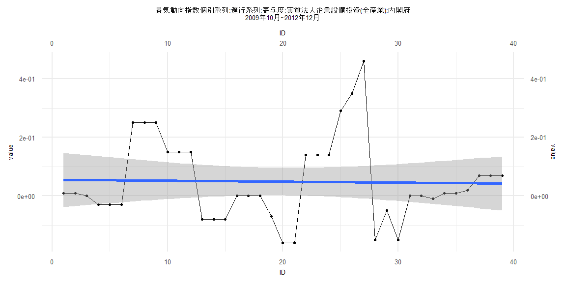
Call:
lm(formula = value ~ ID)

Residuals:
     Min       1Q   Median       3Q      Max
-0.20897 -0.08393 -0.04505  0.09215  0.41326

Coefficients:
              Estimate Std. Error t value Pr(>|t|)
(Intercept)  0.0553711  0.0473791   1.169    0.250
ID          -0.0003198  0.0020645  -0.155    0.878

Residual standard error: 0.1451 on 37 degrees of freedom
Multiple R-squared:  0.0006482, Adjusted R-squared:  -0.02636
F-statistic: 0.024 on 1 and 37 DF,  p-value: 0.8777


    Two-sample Kolmogorov-Smirnov test

data:  lm_residuals and rnorm(n = length(lm_residuals), mean = 0, sd = sd(lm_residuals))
D = 0.33333, p-value = 0.02558
alternative hypothesis: two-sided


    Durbin-Watson test

data:  value ~ ID
DW = 0.90834, p-value = 0.00004184
alternative hypothesis: true autocorrelation is greater than 0


    studentized Breusch-Pagan test

data:  value ~ ID
BP = 0.088426, df = 1, p-value = 0.7662


    Box-Ljung test

data:  lm_residuals
X-squared = 12.455, df = 1, p-value = 0.0004168
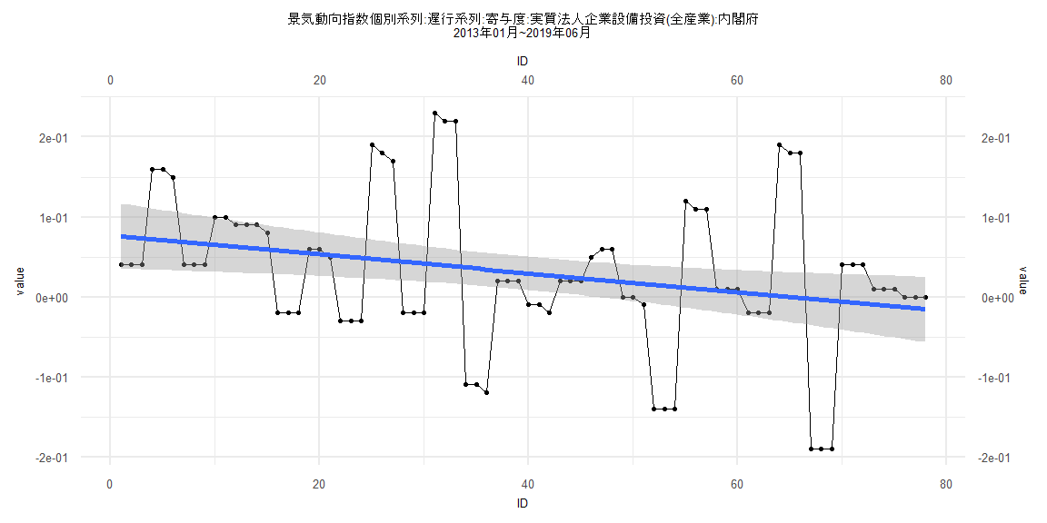
Call:
lm(formula = value ~ ID)

Residuals:
      Min        1Q    Median        3Q       Max
-0.187387 -0.039235 -0.002867  0.038086  0.189752

Coefficients:
              Estimate Std. Error t value Pr(>|t|)
(Intercept)  0.0771562  0.0208781   3.696 0.000412 ***
ID          -0.0011906  0.0004592  -2.593 0.011416 *
---
Signif. codes:  0 '***' 0.001 '**' 0.01 '*' 0.05 '.' 0.1 ' ' 1

Residual standard error: 0.09131 on 76 degrees of freedom
Multiple R-squared:  0.08126,   Adjusted R-squared:  0.06917
F-statistic: 6.722 on 1 and 76 DF,  p-value: 0.01142


    Two-sample Kolmogorov-Smirnov test

data:  lm_residuals and rnorm(n = length(lm_residuals), mean = 0, sd = sd(lm_residuals))
D = 0.11538, p-value = 0.6802
alternative hypothesis: two-sided


    Durbin-Watson test

data:  value ~ ID
DW = 1.0527, p-value = 0.000002206
alternative hypothesis: true autocorrelation is greater than 0


    studentized Breusch-Pagan test

data:  value ~ ID
BP = 2.5415, df = 1, p-value = 0.1109


    Box-Ljung test

data:  lm_residuals
X-squared = 18.089, df = 1, p-value = 0.00002108
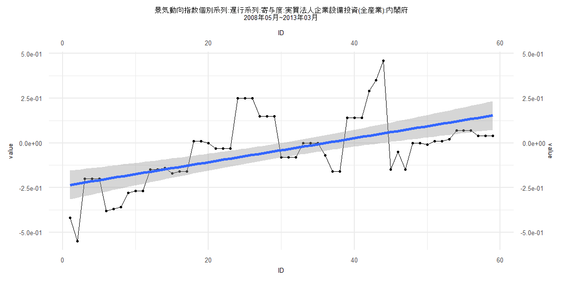
Call:
lm(formula = value ~ ID)

Residuals:
     Min       1Q   Median       3Q      Max
-0.32170 -0.09942 -0.03221  0.08898  0.40687

Coefficients:
             Estimate Std. Error t value    Pr(>|t|)
(Intercept) -0.241701   0.041194  -5.867 0.000000237 ***
ID           0.006701   0.001194   5.611 0.000000617 ***
---
Signif. codes:  0 '***' 0.001 '**' 0.01 '*' 0.05 '.' 0.1 ' ' 1

Residual standard error: 0.1562 on 57 degrees of freedom
Multiple R-squared:  0.3558,    Adjusted R-squared:  0.3445
F-statistic: 31.49 on 1 and 57 DF,  p-value: 0.0000006172


    Two-sample Kolmogorov-Smirnov test

data:  lm_residuals and rnorm(n = length(lm_residuals), mean = 0, sd = sd(lm_residuals))
D = 0.16949, p-value = 0.3674
alternative hypothesis: two-sided


    Durbin-Watson test

data:  value ~ ID
DW = 0.66716, p-value = 0.0000000006401
alternative hypothesis: true autocorrelation is greater than 0


    studentized Breusch-Pagan test

data:  value ~ ID
BP = 0.00002203, df = 1, p-value = 0.9963


    Box-Ljung test

data:  lm_residuals
X-squared = 26.174, df = 1, p-value = 0.0000003119
Call:
lm(formula = value ~ ID)

Residuals:
      Min        1Q    Median        3Q       Max
-0.185767 -0.044733  0.001526  0.038758  0.190314

Coefficients:
              Estimate Std. Error t value Pr(>|t|)
(Intercept)  0.0793766  0.0216601   3.665 0.000467 ***
ID          -0.0013064  0.0004953  -2.638 0.010193 *
---
Signif. codes:  0 '***' 0.001 '**' 0.01 '*' 0.05 '.' 0.1 ' ' 1

Residual standard error: 0.09285 on 73 degrees of freedom
Multiple R-squared:  0.08702,   Adjusted R-squared:  0.07451
F-statistic: 6.958 on 1 and 73 DF,  p-value: 0.01019


    Two-sample Kolmogorov-Smirnov test

data:  lm_residuals and rnorm(n = length(lm_residuals), mean = 0, sd = sd(lm_residuals))
D = 0.16, p-value = 0.2937
alternative hypothesis: two-sided


    Durbin-Watson test

data:  value ~ ID
DW = 1.0364, p-value = 0.000002176
alternative hypothesis: true autocorrelation is greater than 0


    studentized Breusch-Pagan test

data:  value ~ ID
BP = 1.8358, df = 1, p-value = 0.1754


    Box-Ljung test

data:  lm_residuals
X-squared = 17.697, df = 1, p-value = 0.00002591