Analysis
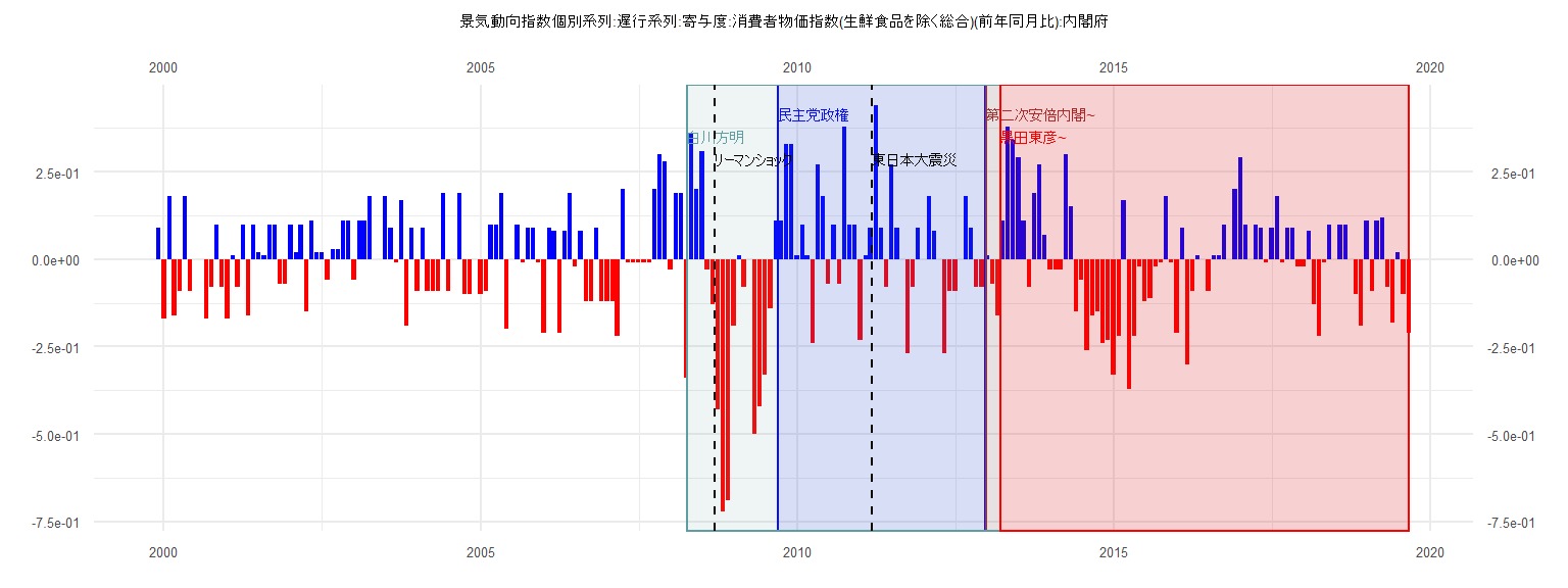
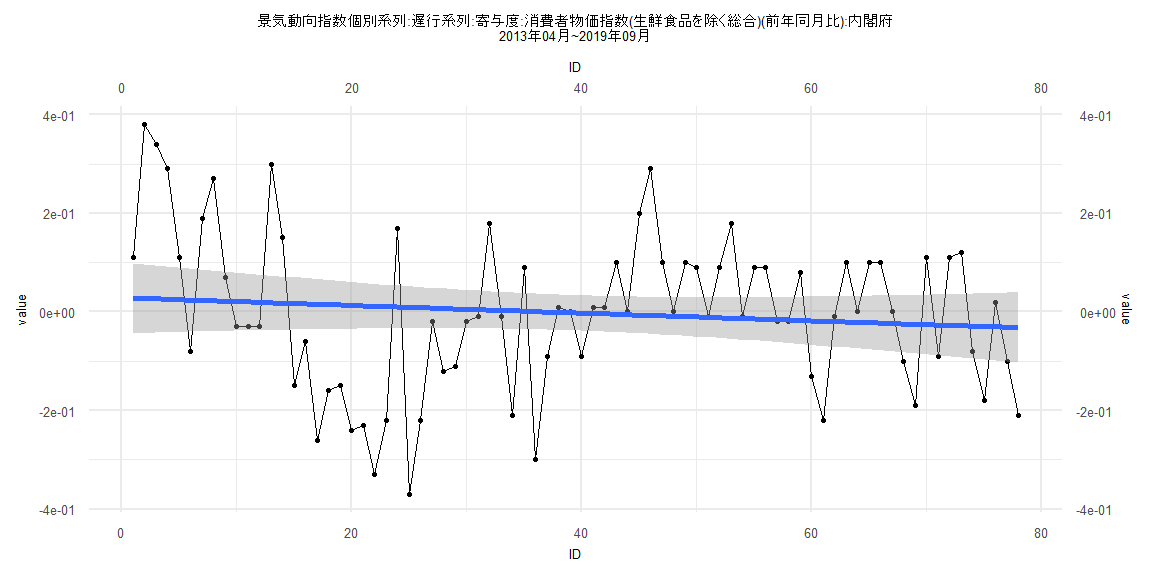
[1] "景気動向指数個別系列:遅行系列:寄与度:消費者物価指数(生鮮食品を除く総合)(前年同月比):内閣府"
       Jan   Feb   Mar   Apr   May   Jun   Jul   Aug   Sep   Oct   Nov   Dec
1999                                                                    0.09
2000 -0.17  0.18 -0.16 -0.09  0.18 -0.09  0.00  0.00 -0.17 -0.08  0.10 -0.08
2001 -0.17  0.01 -0.08  0.10 -0.16  0.10  0.02  0.01  0.10  0.10 -0.07 -0.07
2002  0.10  0.02  0.10 -0.15  0.11  0.02  0.02 -0.06  0.03  0.03  0.11  0.11
2003 -0.06  0.11  0.11  0.18  0.00  0.00  0.18  0.09 -0.01  0.17 -0.19  0.09
2004 -0.09  0.09 -0.09 -0.09 -0.09  0.19 -0.09  0.00  0.19 -0.10 -0.10  0.00
2005 -0.10 -0.09  0.10  0.10  0.19 -0.20  0.00  0.10 -0.01  0.09  0.09 -0.01
2006 -0.21  0.09  0.08 -0.21  0.08  0.19 -0.02  0.08 -0.12 -0.12  0.09 -0.12
2007 -0.12 -0.12 -0.22  0.20 -0.01 -0.01 -0.01 -0.01 -0.01  0.20  0.30  0.28
2008 -0.03  0.19  0.19 -0.34  0.36  0.20  0.31 -0.03 -0.13 -0.43 -0.72 -0.69
2009 -0.19  0.01 -0.08  0.00 -0.50 -0.42 -0.33 -0.14  0.11  0.11  0.33  0.33
2010  0.01  0.10  0.01 -0.24  0.27  0.18 -0.07  0.10 -0.07  0.38  0.10  0.10
2011 -0.23  0.01  0.09  0.44  0.09 -0.08  0.27  0.09  0.00 -0.27 -0.08  0.09
2012  0.00  0.18  0.08  0.00 -0.27 -0.09 -0.09  0.00  0.18  0.09 -0.08 -0.08
2013  0.01 -0.07 -0.16  0.11  0.38  0.34  0.29  0.11 -0.08  0.19  0.27  0.07
2014 -0.03 -0.03 -0.03  0.30  0.15 -0.15 -0.06 -0.26 -0.16 -0.15 -0.24 -0.23
2015 -0.33 -0.22  0.17 -0.37 -0.22 -0.02 -0.12 -0.11 -0.02 -0.01  0.18 -0.01
2016 -0.21  0.09 -0.30 -0.09  0.01  0.00 -0.09  0.01  0.01  0.10  0.00  0.20
2017  0.29  0.10  0.00  0.10  0.09 -0.01  0.09  0.18 -0.01  0.09  0.09 -0.02
2018 -0.02  0.08 -0.13 -0.22 -0.01  0.10  0.00  0.10  0.10  0.00 -0.10 -0.19
2019  0.11 -0.09  0.11  0.12 -0.08 -0.18  0.02 -0.10 -0.21
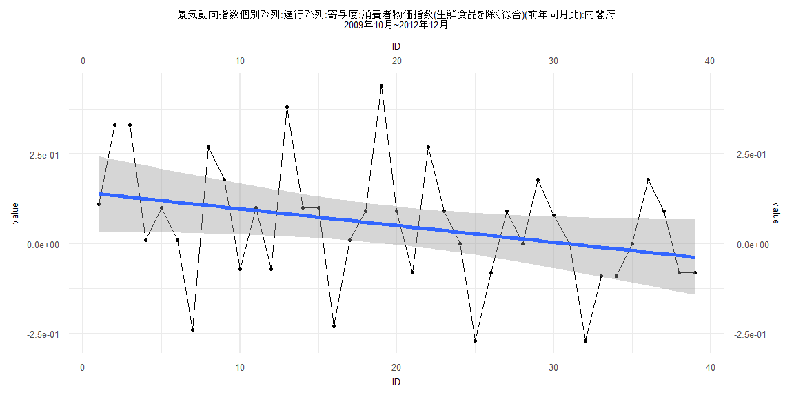
Call:
lm(formula = value ~ ID)

Residuals:
     Min       1Q   Median       3Q      Max
-0.35114 -0.09165  0.00031  0.07691  0.38459

Coefficients:
             Estimate Std. Error t value Pr(>|t|)
(Intercept)  0.143644   0.053651   2.677   0.0110 *
ID          -0.004644   0.002338  -1.986   0.0544 .
---
Signif. codes:  0 '***' 0.001 '**' 0.01 '*' 0.05 '.' 0.1 ' ' 1

Residual standard error: 0.1643 on 37 degrees of freedom
Multiple R-squared:  0.09636,   Adjusted R-squared:  0.07194
F-statistic: 3.946 on 1 and 37 DF,  p-value: 0.05444


    Two-sample Kolmogorov-Smirnov test

data:  lm_residuals and rnorm(n = length(lm_residuals), mean = 0, sd = sd(lm_residuals))
D = 0.15385, p-value = 0.7523
alternative hypothesis: two-sided


    Durbin-Watson test

data:  value ~ ID
DW = 1.8873, p-value = 0.2988
alternative hypothesis: true autocorrelation is greater than 0


    studentized Breusch-Pagan test

data:  value ~ ID
BP = 0.87181, df = 1, p-value = 0.3505


    Box-Ljung test

data:  lm_residuals
X-squared = 0.12731, df = 1, p-value = 0.7212
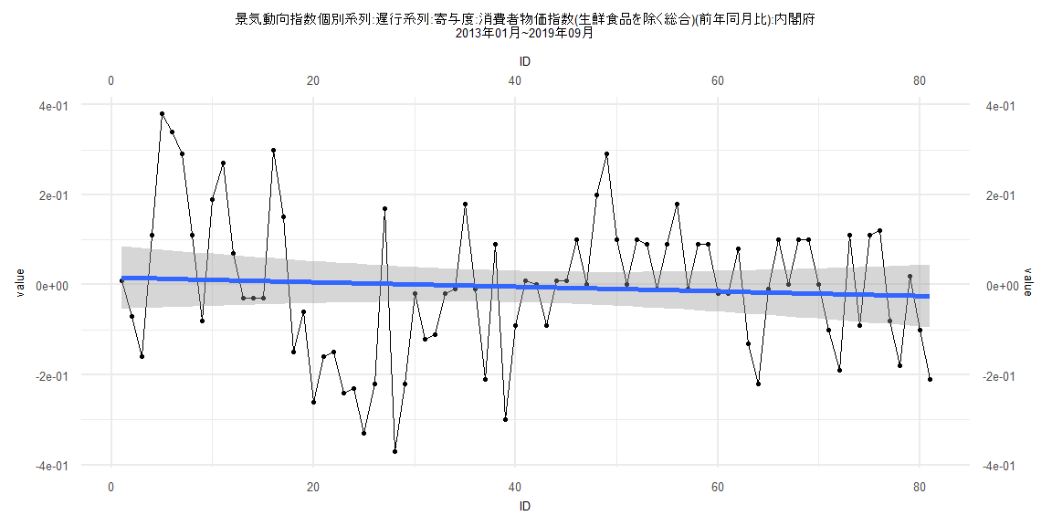
Call:
lm(formula = value ~ ID)

Residuals:
     Min       1Q   Median       3Q      Max
-0.37193 -0.09161  0.00284  0.10724  0.36635

Coefficients:
              Estimate Std. Error t value Pr(>|t|)
(Intercept)  0.0161975  0.0354313   0.457    0.649
ID          -0.0005095  0.0007507  -0.679    0.499

Residual standard error: 0.158 on 79 degrees of freedom
Multiple R-squared:  0.005797,  Adjusted R-squared:  -0.006788
F-statistic: 0.4606 on 1 and 79 DF,  p-value: 0.4993


    Two-sample Kolmogorov-Smirnov test

data:  lm_residuals and rnorm(n = length(lm_residuals), mean = 0, sd = sd(lm_residuals))
D = 0.14815, p-value = 0.338
alternative hypothesis: two-sided


    Durbin-Watson test

data:  value ~ ID
DW = 1.159, p-value = 0.00002039
alternative hypothesis: true autocorrelation is greater than 0


    studentized Breusch-Pagan test

data:  value ~ ID
BP = 8.7705, df = 1, p-value = 0.003061


    Box-Ljung test

data:  lm_residuals
X-squared = 14.252, df = 1, p-value = 0.0001599
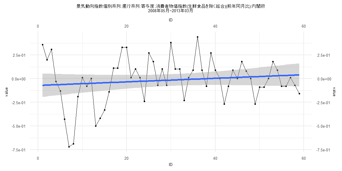
Call:
lm(formula = value ~ ID)

Residuals:
     Min       1Q   Median       3Q      Max
-0.66118 -0.11203  0.01788  0.12486  0.44410

Coefficients:
             Estimate Std. Error t value Pr(>|t|)
(Intercept) -0.072022   0.062819  -1.147    0.256
ID           0.001887   0.001821   1.036    0.305

Residual standard error: 0.2382 on 57 degrees of freedom
Multiple R-squared:  0.01848,   Adjusted R-squared:  0.001263
F-statistic: 1.073 on 1 and 57 DF,  p-value: 0.3046


    Two-sample Kolmogorov-Smirnov test

data:  lm_residuals and rnorm(n = length(lm_residuals), mean = 0, sd = sd(lm_residuals))
D = 0.15254, p-value = 0.5021
alternative hypothesis: two-sided


    Durbin-Watson test

data:  value ~ ID
DW = 0.90192, p-value = 0.0000009176
alternative hypothesis: true autocorrelation is greater than 0


    studentized Breusch-Pagan test

data:  value ~ ID
BP = 10.174, df = 1, p-value = 0.001424


    Box-Ljung test

data:  lm_residuals
X-squared = 16.413, df = 1, p-value = 0.00005094
Call:
lm(formula = value ~ ID)

Residuals:
     Min       1Q   Median       3Q      Max
-0.37922 -0.10046  0.00443  0.10713  0.35291

Coefficients:
              Estimate Std. Error t value Pr(>|t|)
(Intercept)  0.0286480  0.0364351   0.786    0.434
ID          -0.0007772  0.0008014  -0.970    0.335

Residual standard error: 0.1593 on 76 degrees of freedom
Multiple R-squared:  0.01222,   Adjusted R-squared:  -0.0007722
F-statistic: 0.9406 on 1 and 76 DF,  p-value: 0.3352


    Two-sample Kolmogorov-Smirnov test

data:  lm_residuals and rnorm(n = length(lm_residuals), mean = 0, sd = sd(lm_residuals))
D = 0.10256, p-value = 0.81
alternative hypothesis: two-sided


    Durbin-Watson test

data:  value ~ ID
DW = 1.1385, p-value = 0.00001756
alternative hypothesis: true autocorrelation is greater than 0


    studentized Breusch-Pagan test

data:  value ~ ID
BP = 10.586, df = 1, p-value = 0.001139


    Box-Ljung test

data:  lm_residuals
X-squared = 14.348, df = 1, p-value = 0.000152