Analysis
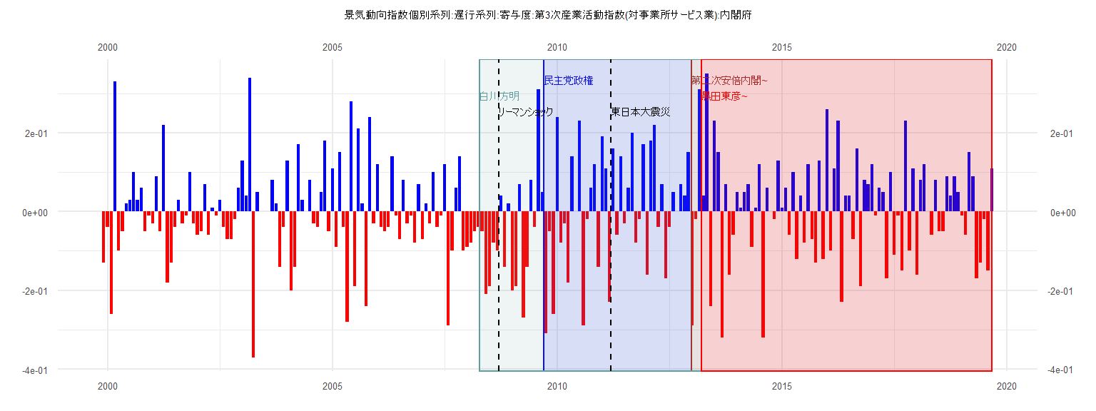
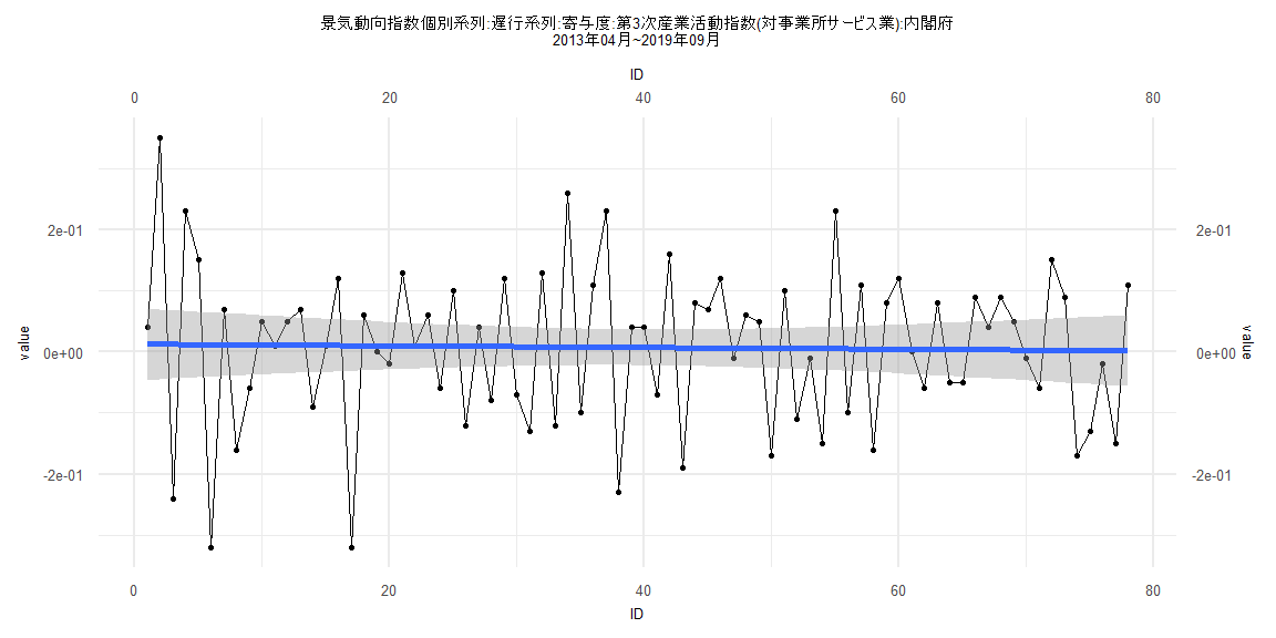
[1] "景気動向指数個別系列:遅行系列:寄与度:第3次産業活動指数(対事業所サービス業):内閣府"
       Jan   Feb   Mar   Apr   May   Jun   Jul   Aug   Sep   Oct   Nov   Dec
1999                                                                   -0.13
2000 -0.04 -0.26  0.33 -0.10 -0.05  0.02  0.03  0.10  0.03  0.06 -0.05 -0.01
2001 -0.03  0.09 -0.05  0.22 -0.18 -0.13 -0.04  0.03 -0.03 -0.01  0.10 -0.03
2002 -0.06 -0.05  0.07 -0.06  0.01 -0.01  0.03 -0.04 -0.07 -0.07 -0.02  0.06
2003  0.13  0.04  0.34 -0.37  0.05  0.00  0.00  0.00  0.08  0.02 -0.14 -0.04
2004  0.13 -0.20 -0.14  0.17  0.03  0.00  0.08 -0.03 -0.04  0.05  0.18 -0.05
2005  0.11 -0.09  0.15 -0.04 -0.28  0.28 -0.19  0.21  0.02 -0.24  0.24 -0.03
2006  0.12 -0.04 -0.05 -0.04  0.14 -0.01 -0.07  0.08 -0.03 -0.01 -0.08  0.07
2007 -0.07  0.02 -0.03  0.10 -0.04 -0.01  0.12 -0.29 -0.10  0.06  0.14 -0.10
2008 -0.09 -0.08 -0.05 -0.04 -0.05 -0.21 -0.19 -0.08 -0.10  0.04 -0.14  0.02
2009 -0.20 -0.19  0.07 -0.27 -0.14  0.08 -0.04  0.31  0.05 -0.31 -0.05 -0.26
2010  0.24 -0.08 -0.03 -0.18  0.14  0.00  0.23 -0.29 -0.02  0.06  0.12 -0.14
2011  0.19  0.11 -0.23  0.16 -0.06  0.14 -0.03  0.06  0.20 -0.08 -0.02  0.17
2012 -0.16  0.18  0.22 -0.04  0.07 -0.17 -0.04  0.05  0.00  0.07  0.04  0.15
2013 -0.29 -0.02  0.31  0.04  0.35 -0.24  0.23  0.15 -0.32  0.07 -0.16 -0.06
2014  0.05  0.01  0.05  0.07 -0.09  0.01  0.12 -0.32  0.06  0.00 -0.02  0.13
2015  0.01  0.06 -0.06  0.10 -0.12  0.04 -0.08  0.12 -0.07 -0.13  0.13 -0.12
2016  0.26 -0.10  0.11  0.23 -0.23  0.04  0.04 -0.07  0.16 -0.19  0.08  0.07
2017  0.12 -0.01  0.06  0.05 -0.17  0.10 -0.11 -0.01 -0.15  0.23 -0.10  0.11
2018 -0.16  0.08  0.12  0.00 -0.06  0.08 -0.05 -0.05  0.09  0.04  0.09  0.05
2019 -0.01 -0.06  0.15  0.09 -0.17 -0.13 -0.02 -0.15  0.11
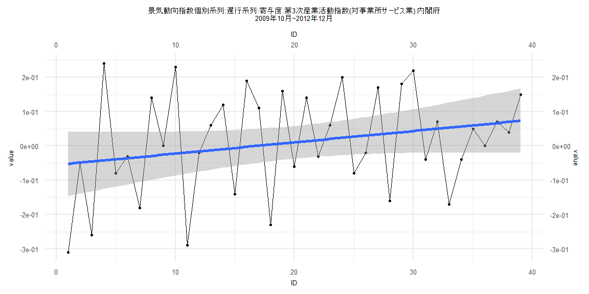
Call:
lm(formula = value ~ ID)

Residuals:
     Min       1Q   Median       3Q      Max
-0.27082 -0.09176 -0.00112  0.12774  0.28228

Coefficients:
             Estimate Std. Error t value Pr(>|t|)
(Intercept) -0.055479   0.048162  -1.152    0.257
ID           0.003300   0.002099   1.572    0.124

Residual standard error: 0.1475 on 37 degrees of freedom
Multiple R-squared:  0.06263,   Adjusted R-squared:  0.03729
F-statistic: 2.472 on 1 and 37 DF,  p-value: 0.1244


    Two-sample Kolmogorov-Smirnov test

data:  lm_residuals and rnorm(n = length(lm_residuals), mean = 0, sd = sd(lm_residuals))
D = 0.15385, p-value = 0.7523
alternative hypothesis: two-sided


    Durbin-Watson test

data:  value ~ ID
DW = 2.6549, p-value = 0.9743
alternative hypothesis: true autocorrelation is greater than 0


    studentized Breusch-Pagan test

data:  value ~ ID
BP = 5.1508, df = 1, p-value = 0.02324


    Box-Ljung test

data:  lm_residuals
X-squared = 5.8349, df = 1, p-value = 0.01571
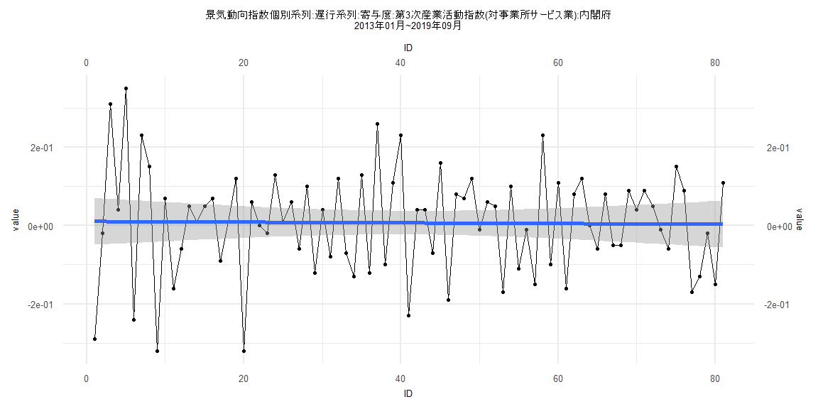
Call:
lm(formula = value ~ ID)

Residuals:
     Min       1Q   Median       3Q      Max
-0.32991 -0.08793  0.02965  0.08610  0.33974

Coefficients:
               Estimate  Std. Error t value Pr(>|t|)
(Intercept)  0.01071296  0.03065365   0.349    0.728
ID          -0.00008966  0.00064947  -0.138    0.891

Residual standard error: 0.1367 on 79 degrees of freedom
Multiple R-squared:  0.0002412, Adjusted R-squared:  -0.01241
F-statistic: 0.01906 on 1 and 79 DF,  p-value: 0.8906


    Two-sample Kolmogorov-Smirnov test

data:  lm_residuals and rnorm(n = length(lm_residuals), mean = 0, sd = sd(lm_residuals))
D = 0.14815, p-value = 0.338
alternative hypothesis: two-sided


    Durbin-Watson test

data:  value ~ ID
DW = 2.6918, p-value = 0.9991
alternative hypothesis: true autocorrelation is greater than 0


    studentized Breusch-Pagan test

data:  value ~ ID
BP = 8.2738, df = 1, p-value = 0.004022


    Box-Ljung test

data:  lm_residuals
X-squared = 12.159, df = 1, p-value = 0.0004884
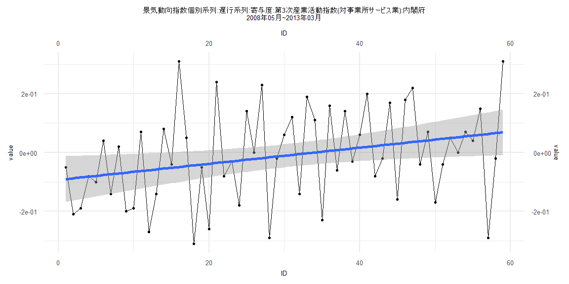
Call:
lm(formula = value ~ ID)

Residuals:
     Min       1Q   Median       3Q      Max
-0.35328 -0.09452 -0.00015  0.12218  0.35903

Coefficients:
             Estimate Std. Error t value Pr(>|t|)
(Intercept) -0.092858   0.039971  -2.323   0.0238 *
ID           0.002739   0.001159   2.364   0.0215 *
---
Signif. codes:  0 '***' 0.001 '**' 0.01 '*' 0.05 '.' 0.1 ' ' 1

Residual standard error: 0.1516 on 57 degrees of freedom
Multiple R-squared:  0.0893,    Adjusted R-squared:  0.07332
F-statistic: 5.589 on 1 and 57 DF,  p-value: 0.0215


    Two-sample Kolmogorov-Smirnov test

data:  lm_residuals and rnorm(n = length(lm_residuals), mean = 0, sd = sd(lm_residuals))
D = 0.11864, p-value = 0.8052
alternative hypothesis: two-sided


    Durbin-Watson test

data:  value ~ ID
DW = 2.4904, p-value = 0.9629
alternative hypothesis: true autocorrelation is greater than 0


    studentized Breusch-Pagan test

data:  value ~ ID
BP = 0.20046, df = 1, p-value = 0.6544


    Box-Ljung test

data:  lm_residuals
X-squared = 4.4578, df = 1, p-value = 0.03474
Call:
lm(formula = value ~ ID)

Residuals:
     Min       1Q   Median       3Q      Max
-0.33190 -0.08632  0.02919  0.08712  0.33755

Coefficients:
              Estimate Std. Error t value Pr(>|t|)
(Intercept)  0.0127273  0.0298399   0.427    0.671
ID          -0.0001372  0.0006563  -0.209    0.835

Residual standard error: 0.1305 on 76 degrees of freedom
Multiple R-squared:  0.0005747, Adjusted R-squared:  -0.01258
F-statistic: 0.0437 on 1 and 76 DF,  p-value: 0.835


    Two-sample Kolmogorov-Smirnov test

data:  lm_residuals and rnorm(n = length(lm_residuals), mean = 0, sd = sd(lm_residuals))
D = 0.21795, p-value = 0.04892
alternative hypothesis: two-sided


    Durbin-Watson test

data:  value ~ ID
DW = 2.8717, p-value = 1
alternative hypothesis: true autocorrelation is greater than 0


    studentized Breusch-Pagan test

data:  value ~ ID
BP = 5.0772, df = 1, p-value = 0.02424


    Box-Ljung test

data:  lm_residuals
X-squared = 15.736, df = 1, p-value = 0.00007284