Analysis
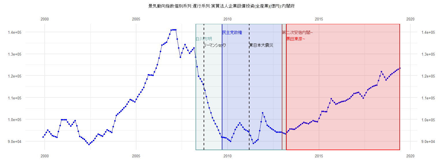
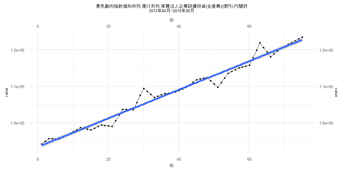
[1] "景気動向指数個別系列:遅行系列:実質法人企業設備投資(全産業)(億円):内閣府"
        Jan    Feb    Mar    Apr    May    Jun    Jul    Aug    Sep    Oct    Nov    Dec
1999                                                                               92001
2000  93043  94084  95126  94264  93402  92540  92299  92057  91816  94501  97185  99870
2001  99846  99821  99797  98833  97869  96905  97771  98637  99503  97072  94641  92210
2002  91771  91331  90892  90119  89345  88572  89154  89735  90317  91299  92282  93264
2003  92945  92625  92306  93302  94297  95293  94898  94503  94108  96697  99286 101875
2004 102516 103157 103798 104526 105254 105982 107030 108078 109126 108764 108402 108040
2005 109197 110355 111512 112547 113582 114617 116555 118494 120432 120342 120253 120163
2006 121814 123465 125116 128097 131079 134060 134483 134905 135328 137196 139065 140933
2007 140959 140985 141011 136851 132690 128530 130457 132383 134310 133004 131699 130393
2008 131180 131966 132753 128430 124107 119784 118572 117360 116148 113292 110435 107579
2009 105304 103030 100755  99408  98060  96713  95139  93565  91991  91825  91658  91492
2010  90982  90471  89961  91775  93588  95402  96412  97422  98432  97447  96462  95477
2011  95099  94721  94343  92581  90819  89057  89616  90175  90734  94830  98926 103022
2012 101141  99260  97379  96804  96230  95655  95177  94699  94221  94209  94198  94186
2013  93909  93632  93355  94122  94889  95656  95611  95566  95521  96022  96523  97024
2014  97571  98118  98665  98455  98246  98036  98496  98955  99415  99263  99110  98958
2015 100530 102101 103673 103632 103591 103550 105508 107466 109424 108600 107775 106951
2016 107290 107630 107969 108114 108260 108405 108829 109254 109678 110386 111095 111803
2017 112018 112232 112447 111539 110632 109724 111009 112294 113579 114062 114544 115027
2018 115266 115504 115743 117804 119866 121927 120650 119373 118096 118868 119640 120412
2019 120948 121484 122020 122505 122990 123475
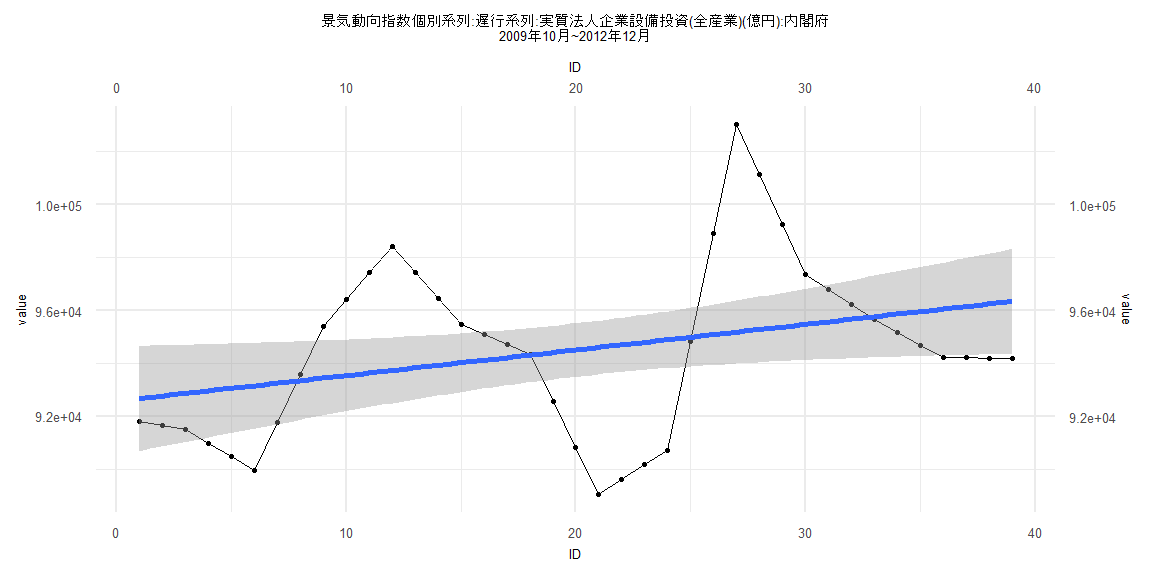
Call:
lm(formula = value ~ ID)

Residuals:
    Min      1Q  Median      3Q     Max
-5549.5 -1962.7  -162.7  1928.8  7836.2

Coefficients:
            Estimate Std. Error t value            Pr(>|t|)
(Intercept) 92578.84    1017.83  90.957 <0.0000000000000002 ***
ID             96.56      44.35   2.177              0.0359 *
---
Signif. codes:  0 '***' 0.001 '**' 0.01 '*' 0.05 '.' 0.1 ' ' 1

Residual standard error: 3117 on 37 degrees of freedom
Multiple R-squared:  0.1136,    Adjusted R-squared:  0.08959
F-statistic:  4.74 on 1 and 37 DF,  p-value: 0.03593


    Two-sample Kolmogorov-Smirnov test

data:  lm_residuals and rnorm(n = length(lm_residuals), mean = 0, sd = sd(lm_residuals))
D = 0.20513, p-value = 0.3888
alternative hypothesis: two-sided


    Durbin-Watson test

data:  value ~ ID
DW = 0.24998, p-value = 0.000000000000001947
alternative hypothesis: true autocorrelation is greater than 0


    studentized Breusch-Pagan test

data:  value ~ ID
BP = 0.37913, df = 1, p-value = 0.5381


    Box-Ljung test

data:  lm_residuals
X-squared = 31.669, df = 1, p-value = 0.00000001829
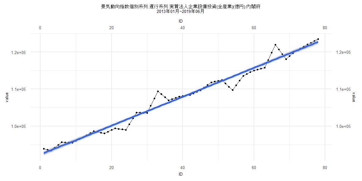
Call:
lm(formula = value ~ ID)

Residuals:
    Min      1Q  Median      3Q     Max
-3652.4  -773.6    76.9   541.5  4236.8

Coefficients:
             Estimate Std. Error t value            Pr(>|t|)
(Intercept) 92318.453    305.622  302.07 <0.0000000000000002 ***
ID            389.961      6.722   58.01 <0.0000000000000002 ***
---
Signif. codes:  0 '***' 0.001 '**' 0.01 '*' 0.05 '.' 0.1 ' ' 1

Residual standard error: 1337 on 76 degrees of freedom
Multiple R-squared:  0.9779,    Adjusted R-squared:  0.9776
F-statistic:  3366 on 1 and 76 DF,  p-value: < 0.00000000000000022


    Two-sample Kolmogorov-Smirnov test

data:  lm_residuals and rnorm(n = length(lm_residuals), mean = 0, sd = sd(lm_residuals))
D = 0.21795, p-value = 0.04892
alternative hypothesis: two-sided


    Durbin-Watson test

data:  value ~ ID
DW = 0.33803, p-value < 0.00000000000000022
alternative hypothesis: true autocorrelation is greater than 0


    studentized Breusch-Pagan test

data:  value ~ ID
BP = 0.72727, df = 1, p-value = 0.3938


    Box-Ljung test

data:  lm_residuals
X-squared = 54.978, df = 1, p-value = 0.0000000000001219
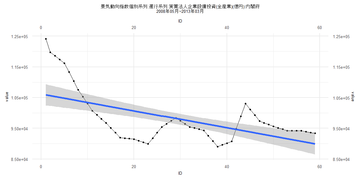
Call:
lm(formula = value ~ ID)

Residuals:
    Min      1Q  Median      3Q     Max
-9900.9 -5093.0  -485.6  3476.4 18181.9

Coefficients:
             Estimate Std. Error t value             Pr(>|t|)
(Intercept) 106200.71    1765.90  60.140 < 0.0000000000000002 ***
ID            -275.60      51.19  -5.384           0.00000143 ***
---
Signif. codes:  0 '***' 0.001 '**' 0.01 '*' 0.05 '.' 0.1 ' ' 1

Residual standard error: 6696 on 57 degrees of freedom
Multiple R-squared:  0.3371,    Adjusted R-squared:  0.3255
F-statistic: 28.99 on 1 and 57 DF,  p-value: 0.000001432


    Two-sample Kolmogorov-Smirnov test

data:  lm_residuals and rnorm(n = length(lm_residuals), mean = 0, sd = sd(lm_residuals))
D = 0.18644, p-value = 0.2582
alternative hypothesis: two-sided


    Durbin-Watson test

data:  value ~ ID
DW = 0.060126, p-value < 0.00000000000000022
alternative hypothesis: true autocorrelation is greater than 0


    studentized Breusch-Pagan test

data:  value ~ ID
BP = 17.743, df = 1, p-value = 0.00002528


    Box-Ljung test

data:  lm_residuals
X-squared = 50.595, df = 1, p-value = 0.000000000001135
Call:
lm(formula = value ~ ID)

Residuals:
    Min      1Q  Median      3Q     Max
-3654.6  -824.3   100.0   542.7  4272.7

Coefficients:
             Estimate Std. Error t value            Pr(>|t|)
(Intercept) 93398.053    315.911  295.65 <0.0000000000000002 ***
ID            391.775      7.223   54.24 <0.0000000000000002 ***
---
Signif. codes:  0 '***' 0.001 '**' 0.01 '*' 0.05 '.' 0.1 ' ' 1

Residual standard error: 1354 on 73 degrees of freedom
Multiple R-squared:  0.9758,    Adjusted R-squared:  0.9755
F-statistic:  2942 on 1 and 73 DF,  p-value: < 0.00000000000000022


    Two-sample Kolmogorov-Smirnov test

data:  lm_residuals and rnorm(n = length(lm_residuals), mean = 0, sd = sd(lm_residuals))
D = 0.17333, p-value = 0.2107
alternative hypothesis: two-sided


    Durbin-Watson test

data:  value ~ ID
DW = 0.3351, p-value < 0.00000000000000022
alternative hypothesis: true autocorrelation is greater than 0


    studentized Breusch-Pagan test

data:  value ~ ID
BP = 0.44422, df = 1, p-value = 0.5051


    Box-Ljung test

data:  lm_residuals
X-squared = 53.794, df = 1, p-value = 0.0000000000002227