Analysis
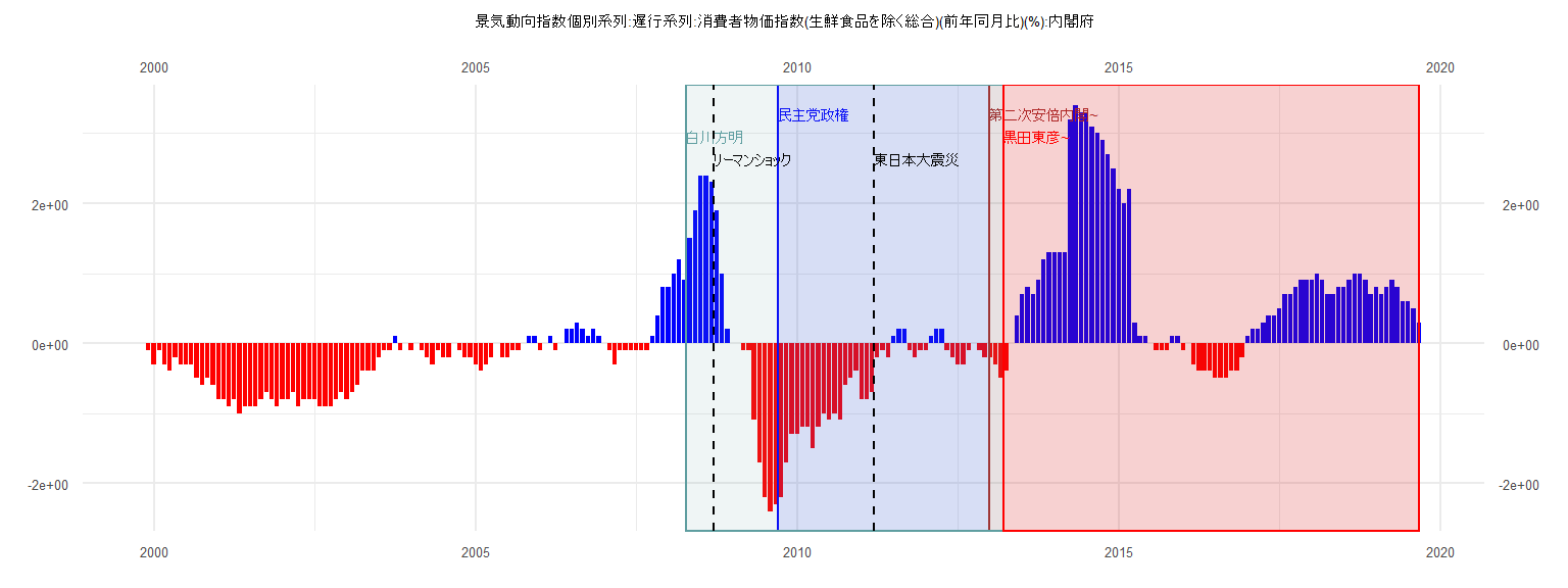
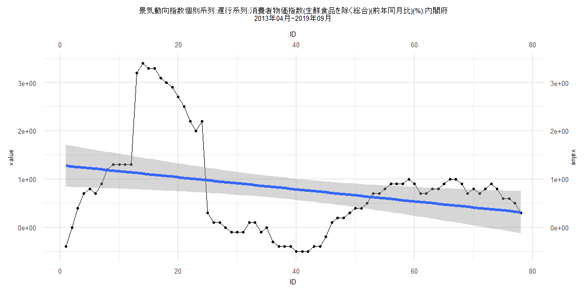
[1] "景気動向指数個別系列:遅行系列:消費者物価指数(生鮮食品を除く総合)(前年同月比)(%):内閣府"
      Jan  Feb  Mar  Apr  May  Jun  Jul  Aug  Sep  Oct  Nov  Dec
1999                                                        -0.1
2000 -0.3 -0.1 -0.3 -0.4 -0.2 -0.3 -0.3 -0.3 -0.5 -0.6 -0.5 -0.6
2001 -0.8 -0.8 -0.9 -0.8 -1.0 -0.9 -0.9 -0.9 -0.8 -0.7 -0.8 -0.9
2002 -0.8 -0.8 -0.7 -0.9 -0.8 -0.8 -0.8 -0.9 -0.9 -0.9 -0.8 -0.7
2003 -0.8 -0.7 -0.6 -0.4 -0.4 -0.4 -0.2 -0.1 -0.1  0.1 -0.1  0.0
2004 -0.1  0.0 -0.1 -0.2 -0.3 -0.1 -0.2 -0.2  0.0 -0.1 -0.2 -0.2
2005 -0.3 -0.4 -0.3 -0.2  0.0 -0.2 -0.2 -0.1 -0.1  0.0  0.1  0.1
2006 -0.1  0.0  0.1 -0.1  0.0  0.2  0.2  0.3  0.2  0.1  0.2  0.1
2007  0.0 -0.1 -0.3 -0.1 -0.1 -0.1 -0.1 -0.1 -0.1  0.1  0.4  0.8
2008  0.8  1.0  1.2  0.9  1.5  1.9  2.4  2.4  2.3  1.9  1.0  0.2
2009  0.0  0.0 -0.1 -0.1 -1.1 -1.7 -2.2 -2.4 -2.3 -2.2 -1.7 -1.3
2010 -1.3 -1.2 -1.2 -1.5 -1.2 -1.0 -1.1 -1.0 -1.1 -0.6 -0.5 -0.4
2011 -0.8 -0.8 -0.7 -0.2 -0.1 -0.2  0.1  0.2  0.2 -0.1 -0.2 -0.1
2012 -0.1  0.1  0.2  0.2 -0.1 -0.2 -0.3 -0.3 -0.1  0.0 -0.1 -0.2
2013 -0.2 -0.3 -0.5 -0.4  0.0  0.4  0.7  0.8  0.7  0.9  1.2  1.3
2014  1.3  1.3  1.3  3.2  3.4  3.3  3.3  3.1  3.0  2.9  2.7  2.5
2015  2.2  2.0  2.2  0.3  0.1  0.1  0.0 -0.1 -0.1 -0.1  0.1  0.1
2016 -0.1  0.0 -0.3 -0.4 -0.4 -0.4 -0.5 -0.5 -0.5 -0.4 -0.4 -0.2
2017  0.1  0.2  0.2  0.3  0.4  0.4  0.5  0.7  0.7  0.8  0.9  0.9
2018  0.9  1.0  0.9  0.7  0.7  0.8  0.8  0.9  1.0  1.0  0.9  0.7
2019  0.8  0.7  0.8  0.9  0.8  0.6  0.6  0.5  0.3
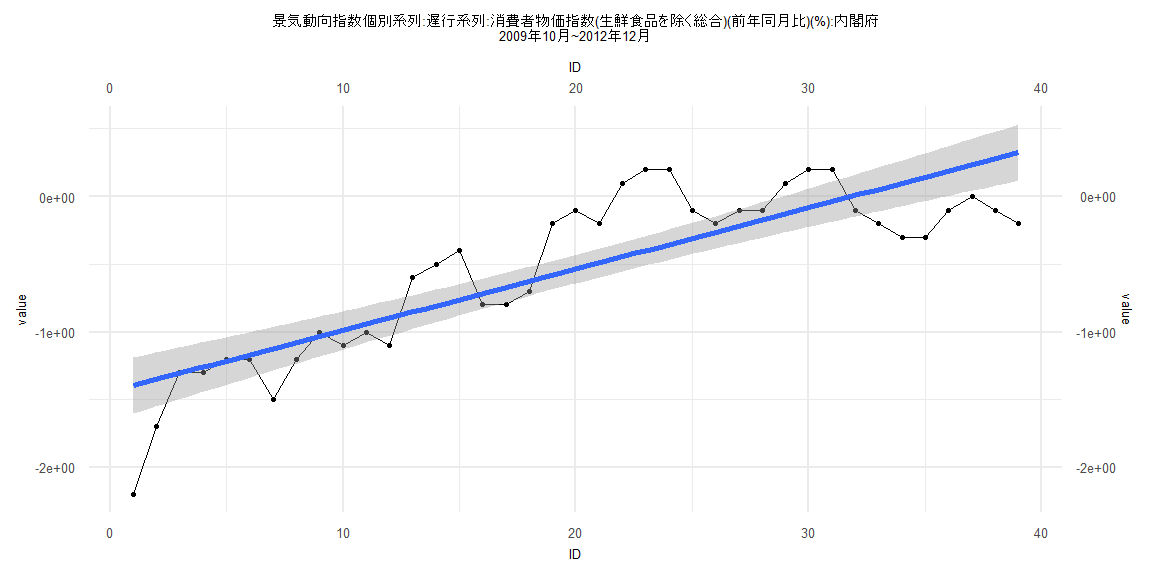
Call:
lm(formula = value ~ ID)

Residuals:
     Min       1Q   Median       3Q      Max
-0.80333 -0.21797 -0.02985  0.24529  0.59999

Coefficients:
             Estimate Std. Error t value             Pr(>|t|)
(Intercept) -1.441970   0.106425 -13.549 0.000000000000000643 ***
ID           0.045304   0.004637   9.769 0.000000000008637938 ***
---
Signif. codes:  0 '***' 0.001 '**' 0.01 '*' 0.05 '.' 0.1 ' ' 1

Residual standard error: 0.3259 on 37 degrees of freedom
Multiple R-squared:  0.7206,    Adjusted R-squared:  0.7131
F-statistic: 95.44 on 1 and 37 DF,  p-value: 0.000000000008638


    Two-sample Kolmogorov-Smirnov test

data:  lm_residuals and rnorm(n = length(lm_residuals), mean = 0, sd = sd(lm_residuals))
D = 0.15385, p-value = 0.7523
alternative hypothesis: two-sided


    Durbin-Watson test

data:  value ~ ID
DW = 0.43675, p-value = 0.0000000001134
alternative hypothesis: true autocorrelation is greater than 0


    studentized Breusch-Pagan test

data:  value ~ ID
BP = 0.082674, df = 1, p-value = 0.7737


    Box-Ljung test

data:  lm_residuals
X-squared = 18.58, df = 1, p-value = 0.00001629
Call:
lm(formula = value ~ ID)

Residuals:
     Min       1Q   Median       3Q      Max
-1.56452 -0.77767  0.06985  0.32722  2.45022

Coefficients:
             Estimate Std. Error t value  Pr(>|t|)
(Intercept)  1.089105   0.224789   4.845 0.0000062 ***
ID          -0.008196   0.004763  -1.721    0.0892 .
---
Signif. codes:  0 '***' 0.001 '**' 0.01 '*' 0.05 '.' 0.1 ' ' 1

Residual standard error: 1.002 on 79 degrees of freedom
Multiple R-squared:  0.03613,   Adjusted R-squared:  0.02393
F-statistic: 2.961 on 1 and 79 DF,  p-value: 0.0892


    Two-sample Kolmogorov-Smirnov test

data:  lm_residuals and rnorm(n = length(lm_residuals), mean = 0, sd = sd(lm_residuals))
D = 0.12346, p-value = 0.5705
alternative hypothesis: two-sided


    Durbin-Watson test

data:  value ~ ID
DW = 0.11347, p-value < 0.00000000000000022
alternative hypothesis: true autocorrelation is greater than 0


    studentized Breusch-Pagan test

data:  value ~ ID
BP = 18.231, df = 1, p-value = 0.00001957


    Box-Ljung test

data:  lm_residuals
X-squared = 73.127, df = 1, p-value < 0.00000000000000022
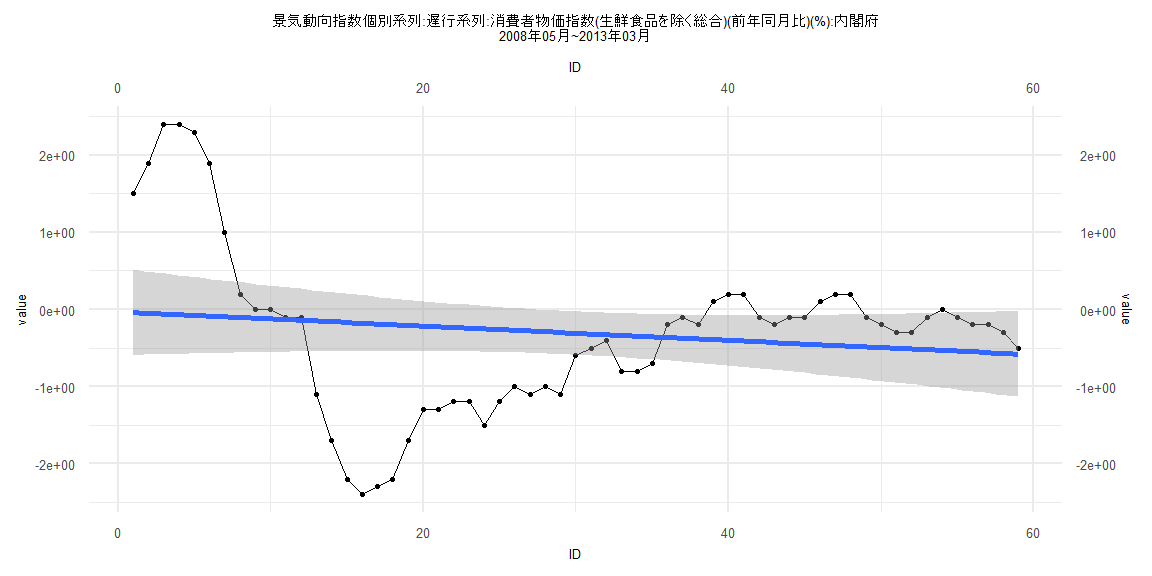
Call:
lm(formula = value ~ ID)

Residuals:
    Min      1Q  Median      3Q     Max
-2.2217 -0.7648  0.1829  0.4316  2.4667

Coefficients:
             Estimate Std. Error t value Pr(>|t|)
(Intercept) -0.029515   0.283536  -0.104    0.917
ID          -0.009299   0.008219  -1.131    0.263

Residual standard error: 1.075 on 57 degrees of freedom
Multiple R-squared:  0.02196,   Adjusted R-squared:  0.004802
F-statistic:  1.28 on 1 and 57 DF,  p-value: 0.2627


    Two-sample Kolmogorov-Smirnov test

data:  lm_residuals and rnorm(n = length(lm_residuals), mean = 0, sd = sd(lm_residuals))
D = 0.16949, p-value = 0.3674
alternative hypothesis: two-sided


    Durbin-Watson test

data:  value ~ ID
DW = 0.08481, p-value < 0.00000000000000022
alternative hypothesis: true autocorrelation is greater than 0


    studentized Breusch-Pagan test

data:  value ~ ID
BP = 23.199, df = 1, p-value = 0.000001461


    Box-Ljung test

data:  lm_residuals
X-squared = 54.78, df = 1, p-value = 0.0000000000001348
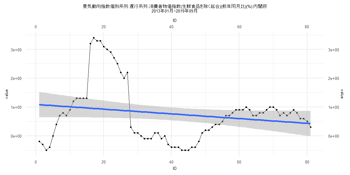
Call:
lm(formula = value ~ ID)

Residuals:
    Min      1Q  Median      3Q     Max
-1.6765 -0.8512  0.1051  0.4054  2.2862

Coefficients:
             Estimate Std. Error t value    Pr(>|t|)
(Intercept)  1.288978   0.223186   5.775 0.000000159 ***
ID          -0.012509   0.004909  -2.548      0.0128 *
---
Signif. codes:  0 '***' 0.001 '**' 0.01 '*' 0.05 '.' 0.1 ' ' 1

Residual standard error: 0.9761 on 76 degrees of freedom
Multiple R-squared:  0.07872,   Adjusted R-squared:  0.06659
F-statistic: 6.494 on 1 and 76 DF,  p-value: 0.01284


    Two-sample Kolmogorov-Smirnov test

data:  lm_residuals and rnorm(n = length(lm_residuals), mean = 0, sd = sd(lm_residuals))
D = 0.21795, p-value = 0.04892
alternative hypothesis: two-sided


    Durbin-Watson test

data:  value ~ ID
DW = 0.12373, p-value < 0.00000000000000022
alternative hypothesis: true autocorrelation is greater than 0


    studentized Breusch-Pagan test

data:  value ~ ID
BP = 18.53, df = 1, p-value = 0.00001673


    Box-Ljung test

data:  lm_residuals
X-squared = 68.402, df = 1, p-value < 0.00000000000000022