Analysis
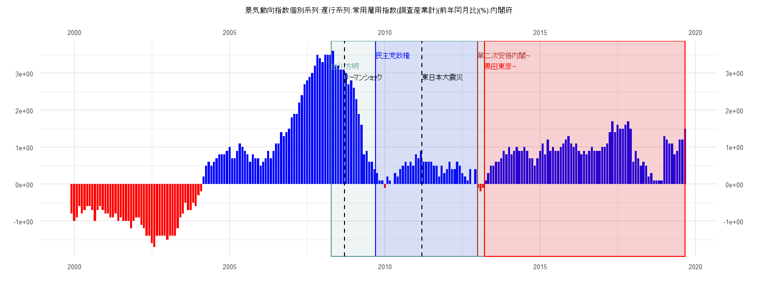
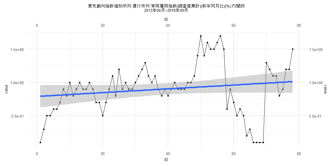
[1] "景気動向指数個別系列:遅行系列:常用雇用指数(調査産業計)(前年同月比)(%):内閣府"
      Jan  Feb  Mar  Apr  May  Jun  Jul  Aug  Sep  Oct  Nov  Dec
1999                                                        -0.8
2000 -1.0 -0.9 -0.6 -0.8 -0.7 -0.6 -0.6 -0.7 -1.0 -0.7 -0.6 -0.7
2001 -0.8 -0.8 -0.9 -0.9 -0.8 -1.0 -0.9 -1.0 -1.0 -1.0 -1.2 -1.0
2002 -0.9 -0.9 -1.1 -1.2 -1.4 -1.4 -1.6 -1.7 -1.4 -1.4 -1.4 -1.4
2003 -1.5 -1.4 -1.4 -1.4 -1.2 -0.9 -0.8 -0.5 -0.7 -0.7 -0.5 -0.6
2004 -0.3 -0.2  0.2  0.5  0.6  0.5  0.6  0.7  0.8  0.8  0.8  0.9
2005  1.0  0.7  0.7  0.9  1.1  1.0  0.9  0.8  0.6  0.8  0.7  0.7
2006  0.5  0.6  0.7  0.9  0.7  0.9  1.1  1.1  1.4  1.3  1.4  1.5
2007  1.8  1.9  1.9  2.2  2.4  2.7  2.8  2.9  3.0  3.2  3.5  3.4
2008  3.3  3.5  3.5  3.5  3.6  3.2  3.2  3.1  3.1  3.0  2.7  2.8
2009  2.6  2.3  1.9  1.6  0.8  0.9  0.6  0.6  0.4  0.3  0.1  0.1
2010 -0.1  0.2  0.1  0.0  0.3  0.2  0.4  0.5  0.6  0.5  0.6  0.5
2011  0.8  0.7  0.9  0.6  0.6  0.6  0.6  0.5  0.5  0.2  0.5  0.3
2012  0.4  0.6  0.4  0.4  0.6  0.5  0.3  0.2  0.1  0.4  0.0  0.4
2013 -0.1 -0.2 -0.1  0.1  0.3  0.5  0.5  0.6  0.6  0.7  0.9  0.8
2014  1.0  0.8  0.9  1.0  0.9  0.9  1.0  0.9  0.7  0.7  0.5  0.7
2015  0.9  1.1  0.8  1.2  0.9  1.0  0.9  0.9  1.0  1.1  1.2  1.3
2016  1.1  1.0  1.1  0.9  0.8  0.9  0.8  0.9  1.0  0.9  0.9  0.9
2017  1.0  1.0  1.1  1.4  1.7  1.4  1.6  1.5  1.5  1.6  1.7  1.5
2018  0.6  0.9  0.7  0.5  0.6  0.5  0.2  0.3  0.1  0.1  0.1  0.1
2019  1.3  1.2  1.1  1.1  0.8  0.9  1.2  1.2  1.5
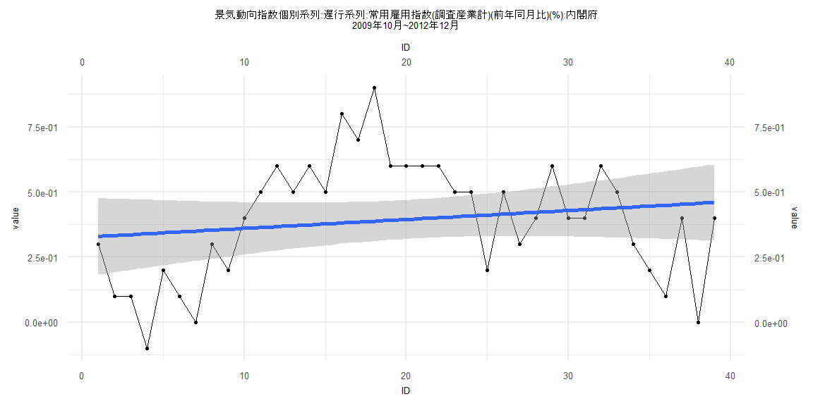
Call:
lm(formula = value ~ ID)

Residuals:
     Min       1Q   Median       3Q      Max
-0.45645 -0.15040 -0.02224  0.16921  0.51197

Coefficients:
            Estimate Std. Error t value Pr(>|t|)
(Intercept) 0.326451   0.075173   4.343 0.000105 ***
ID          0.003421   0.003276   1.044 0.303075
---
Signif. codes:  0 '***' 0.001 '**' 0.01 '*' 0.05 '.' 0.1 ' ' 1

Residual standard error: 0.2302 on 37 degrees of freedom
Multiple R-squared:  0.02864,   Adjusted R-squared:  0.002383
F-statistic: 1.091 on 1 and 37 DF,  p-value: 0.3031


    Two-sample Kolmogorov-Smirnov test

data:  lm_residuals and rnorm(n = length(lm_residuals), mean = 0, sd = sd(lm_residuals))
D = 0.15385, p-value = 0.7523
alternative hypothesis: two-sided


    Durbin-Watson test

data:  value ~ ID
DW = 0.73924, p-value = 0.000001452
alternative hypothesis: true autocorrelation is greater than 0


    studentized Breusch-Pagan test

data:  value ~ ID
BP = 0.33666, df = 1, p-value = 0.5618


    Box-Ljung test

data:  lm_residuals
X-squared = 16.661, df = 1, p-value = 0.00004469
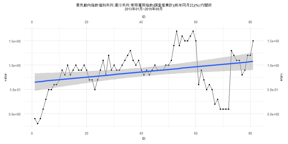
Call:
lm(formula = value ~ ID)

Residuals:
     Min       1Q   Median       3Q      Max
-0.92911 -0.16079  0.08209  0.24513  0.77121

Coefficients:
            Estimate Std. Error t value       Pr(>|t|)
(Intercept) 0.648951   0.091157   7.119 0.000000000442 ***
ID          0.005280   0.001931   2.734        0.00772 **
---
Signif. codes:  0 '***' 0.001 '**' 0.01 '*' 0.05 '.' 0.1 ' ' 1

Residual standard error: 0.4064 on 79 degrees of freedom
Multiple R-squared:  0.08643,   Adjusted R-squared:  0.07486
F-statistic: 7.474 on 1 and 79 DF,  p-value: 0.007724


    Two-sample Kolmogorov-Smirnov test

data:  lm_residuals and rnorm(n = length(lm_residuals), mean = 0, sd = sd(lm_residuals))
D = 0.22222, p-value = 0.03633
alternative hypothesis: two-sided


    Durbin-Watson test

data:  value ~ ID
DW = 0.33454, p-value < 0.00000000000000022
alternative hypothesis: true autocorrelation is greater than 0


    studentized Breusch-Pagan test

data:  value ~ ID
BP = 4.3968, df = 1, p-value = 0.03601


    Box-Ljung test

data:  lm_residuals
X-squared = 54.332, df = 1, p-value = 0.0000000000001693
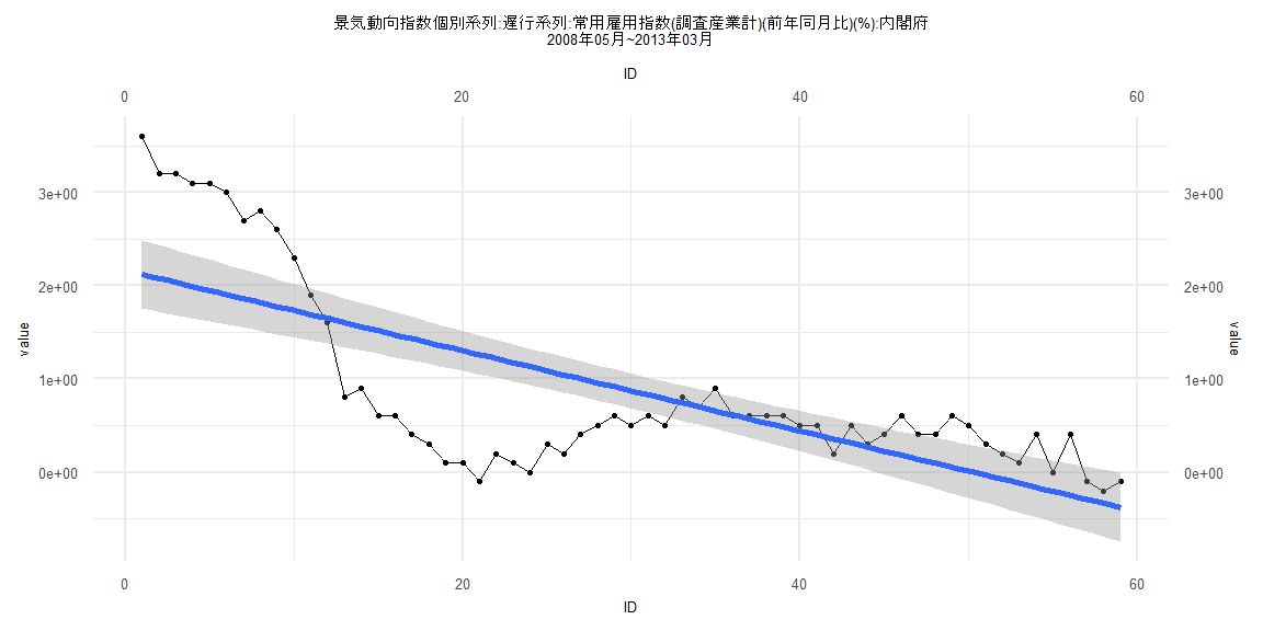
Call:
lm(formula = value ~ ID)

Residuals:
    Min      1Q  Median      3Q     Max
-1.3587 -0.5288  0.1025  0.3755  1.4800

Coefficients:
             Estimate Std. Error t value             Pr(>|t|)
(Intercept)  2.163063   0.188085  11.500 < 0.0000000000000002 ***
ID          -0.043063   0.005452  -7.898       0.000000000102 ***
---
Signif. codes:  0 '***' 0.001 '**' 0.01 '*' 0.05 '.' 0.1 ' ' 1

Residual standard error: 0.7132 on 57 degrees of freedom
Multiple R-squared:  0.5225,    Adjusted R-squared:  0.5142
F-statistic: 62.38 on 1 and 57 DF,  p-value: 0.0000000001015


    Two-sample Kolmogorov-Smirnov test

data:  lm_residuals and rnorm(n = length(lm_residuals), mean = 0, sd = sd(lm_residuals))
D = 0.10169, p-value = 0.9239
alternative hypothesis: two-sided


    Durbin-Watson test

data:  value ~ ID
DW = 0.10206, p-value < 0.00000000000000022
alternative hypothesis: true autocorrelation is greater than 0


    studentized Breusch-Pagan test

data:  value ~ ID
BP = 28.248, df = 1, p-value = 0.0000001068


    Box-Ljung test

data:  lm_residuals
X-squared = 51.37, df = 1, p-value = 0.0000000000007649
Call:
lm(formula = value ~ ID)

Residuals:
     Min       1Q   Median       3Q      Max
-0.88774 -0.14981  0.04024  0.19164  0.76629

Coefficients:
            Estimate Std. Error t value           Pr(>|t|)
(Intercept) 0.791508   0.086390   9.162 0.0000000000000654 ***
ID          0.002844   0.001900   1.497              0.139
---
Signif. codes:  0 '***' 0.001 '**' 0.01 '*' 0.05 '.' 0.1 ' ' 1

Residual standard error: 0.3778 on 76 degrees of freedom
Multiple R-squared:  0.02863,   Adjusted R-squared:  0.01585
F-statistic:  2.24 on 1 and 76 DF,  p-value: 0.1386


    Two-sample Kolmogorov-Smirnov test

data:  lm_residuals and rnorm(n = length(lm_residuals), mean = 0, sd = sd(lm_residuals))
D = 0.10256, p-value = 0.81
alternative hypothesis: two-sided


    Durbin-Watson test

data:  value ~ ID
DW = 0.39752, p-value < 0.00000000000000022
alternative hypothesis: true autocorrelation is greater than 0


    studentized Breusch-Pagan test

data:  value ~ ID
BP = 11.84, df = 1, p-value = 0.0005796


    Box-Ljung test

data:  lm_residuals
X-squared = 47.812, df = 1, p-value = 0.000000000004691