Analysis
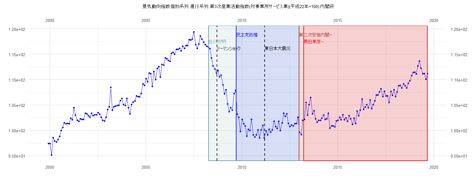
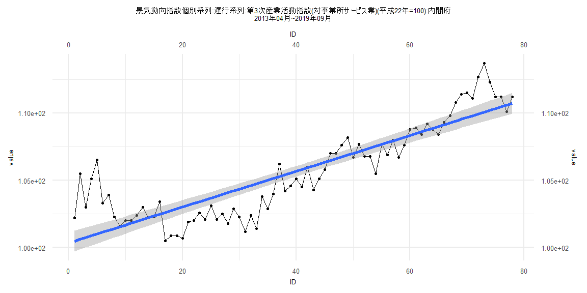
[1] "景気動向指数個別系列:遅行系列:第3次産業活動指数(対事業所サービス業)(平成22年=100):内閣府"
       Jan   Feb   Mar   Apr   May   Jun   Jul   Aug   Sep   Oct   Nov   Dec
1999                                                                    97.4
2000  97.4  95.2  98.6  97.9  97.7  98.2  98.8 100.0 100.6 101.5 101.3 101.4
2001 101.3 102.4 102.1 104.5 103.0 102.0 101.8 102.3 102.2 102.2 103.4 103.3
2002 102.9 102.6 103.4 102.9 103.1 103.1 103.5 103.2 102.6 102.0 101.9 102.6
2003 104.1 104.7 108.5 104.0 104.7 104.8 104.9 105.0 105.9 106.3 105.1 104.9
2004 106.3 104.5 103.3 105.1 105.6 105.8 106.8 106.7 106.6 107.3 109.2 108.9
2005 110.2 109.6 111.3 111.2 108.7 111.6 110.0 112.2 112.6 110.5 113.0 112.9
2006 114.3 114.1 113.8 113.6 115.2 115.4 115.0 116.0 116.0 116.2 115.7 116.6
2007 116.2 116.7 116.7 117.9 117.8 118.0 119.4 116.9 116.2 117.0 118.6 118.0
2008 117.4 116.9 116.6 116.4 116.1 114.3 112.7 112.1 111.3 111.8 110.6 110.9
2009 109.0 107.2 108.0 105.2 103.7 104.5 104.0 107.3 107.9 103.2 102.6  99.8
2010 102.2 101.3 100.9  98.9 100.2 100.0 102.2  99.1  98.7  99.1 100.1  98.5
2011 100.1 101.0  98.5  99.9  99.1 100.2  99.7 100.1 101.8 100.8 100.4 101.8
2012 100.0 101.5 103.4 102.8 103.3 101.4 100.8 101.1 100.9 101.3 101.4 102.6
2013  99.6  99.2 102.0 102.2 105.5 103.0 105.1 106.5 103.3 103.9 102.3 101.6
2014 102.0 102.0 102.4 103.0 102.2 102.3 103.4 100.5 100.9 100.9 100.7 101.9
2015 102.0 102.6 102.1 103.1 102.1 102.5 101.8 102.9 102.3 101.2 102.4 101.4
2016 103.8 102.9 104.0 106.2 104.2 104.6 105.1 104.5 106.0 104.3 105.1 105.8
2017 107.0 107.0 107.6 108.2 106.7 107.7 106.8 106.8 105.5 107.7 106.9 108.0
2018 106.7 107.6 108.8 108.9 108.4 109.2 108.8 108.4 109.3 109.8 110.8 111.4
2019 111.5 111.1 112.7 113.7 112.3 111.2 111.2 110.1 111.2
Call:
lm(formula = value ~ ID)

Residuals:
    Min      1Q  Median      3Q     Max
-2.2261 -0.8177 -0.2209  0.8449  2.9928

Coefficients:
             Estimate Std. Error t value            Pr(>|t|)
(Intercept) 100.17665    0.43721 229.126 <0.0000000000000002 ***
ID            0.03053    0.01905   1.602               0.118
---
Signif. codes:  0 '***' 0.001 '**' 0.01 '*' 0.05 '.' 0.1 ' ' 1

Residual standard error: 1.339 on 37 degrees of freedom
Multiple R-squared:  0.06489,   Adjusted R-squared:  0.03961
F-statistic: 2.567 on 1 and 37 DF,  p-value: 0.1176


    Two-sample Kolmogorov-Smirnov test

data:  lm_residuals and rnorm(n = length(lm_residuals), mean = 0, sd = sd(lm_residuals))
D = 0.20513, p-value = 0.3888
alternative hypothesis: two-sided


    Durbin-Watson test

data:  value ~ ID
DW = 1.1205, p-value = 0.0009629
alternative hypothesis: true autocorrelation is greater than 0


    studentized Breusch-Pagan test

data:  value ~ ID
BP = 4.5864, df = 1, p-value = 0.03223


    Box-Ljung test

data:  lm_residuals
X-squared = 5.4778, df = 1, p-value = 0.01926
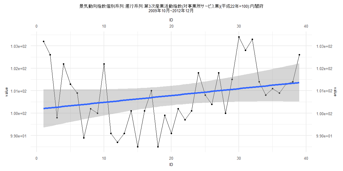
Call:
lm(formula = value ~ ID)

Residuals:
    Min      1Q  Median      3Q     Max
-3.3461 -1.2111 -0.0521  0.8679  5.4779

Coefficients:
             Estimate Std. Error t value            Pr(>|t|)
(Intercept) 99.958148   0.383627  260.56 <0.0000000000000002 ***
ID           0.132999   0.008128   16.36 <0.0000000000000002 ***
---
Signif. codes:  0 '***' 0.001 '**' 0.01 '*' 0.05 '.' 0.1 ' ' 1

Residual standard error: 1.71 on 79 degrees of freedom
Multiple R-squared:  0.7722,    Adjusted R-squared:  0.7693
F-statistic: 267.7 on 1 and 79 DF,  p-value: < 0.00000000000000022


    Two-sample Kolmogorov-Smirnov test

data:  lm_residuals and rnorm(n = length(lm_residuals), mean = 0, sd = sd(lm_residuals))
D = 0.08642, p-value = 0.9254
alternative hypothesis: two-sided


    Durbin-Watson test

data:  value ~ ID
DW = 0.51825, p-value < 0.00000000000000022
alternative hypothesis: true autocorrelation is greater than 0


    studentized Breusch-Pagan test

data:  value ~ ID
BP = 6.0736, df = 1, p-value = 0.01372


    Box-Ljung test

data:  lm_residuals
X-squared = 46.003, df = 1, p-value = 0.0000000000118
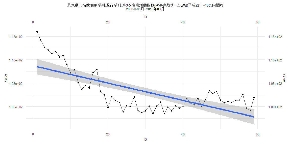
Call:
lm(formula = value ~ ID)

Residuals:
    Min      1Q  Median      3Q     Max
-5.3970 -2.6254 -0.1705  2.4283  7.5525

Coefficients:
             Estimate Std. Error t value             Pr(>|t|)
(Intercept) 108.73226    0.83754 129.824 < 0.0000000000000002 ***
ID           -0.18480    0.02428  -7.612       0.000000000304 ***
---
Signif. codes:  0 '***' 0.001 '**' 0.01 '*' 0.05 '.' 0.1 ' ' 1

Residual standard error: 3.176 on 57 degrees of freedom
Multiple R-squared:  0.5041,    Adjusted R-squared:  0.4954
F-statistic: 57.94 on 1 and 57 DF,  p-value: 0.0000000003042


    Two-sample Kolmogorov-Smirnov test

data:  lm_residuals and rnorm(n = length(lm_residuals), mean = 0, sd = sd(lm_residuals))
D = 0.10169, p-value = 0.9239
alternative hypothesis: two-sided


    Durbin-Watson test

data:  value ~ ID
DW = 0.25817, p-value < 0.00000000000000022
alternative hypothesis: true autocorrelation is greater than 0


    studentized Breusch-Pagan test

data:  value ~ ID
BP = 7.943, df = 1, p-value = 0.004827


    Box-Ljung test

data:  lm_residuals
X-squared = 40.328, df = 1, p-value = 0.0000000002147
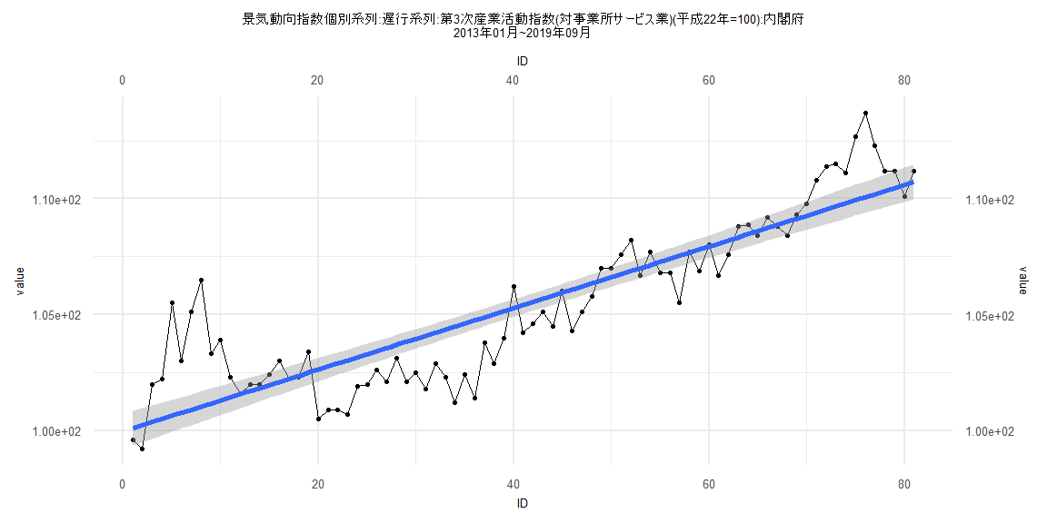
Call:
lm(formula = value ~ ID)

Residuals:
    Min      1Q  Median      3Q     Max
-3.3440 -1.2376 -0.0321  0.8651  5.4821

Coefficients:
              Estimate Std. Error t value            Pr(>|t|)
(Intercept) 100.352481   0.395262  253.89 <0.0000000000000002 ***
ID            0.133076   0.008694   15.31 <0.0000000000000002 ***
---
Signif. codes:  0 '***' 0.001 '**' 0.01 '*' 0.05 '.' 0.1 ' ' 1

Residual standard error: 1.729 on 76 degrees of freedom
Multiple R-squared:  0.7551,    Adjusted R-squared:  0.7519
F-statistic: 234.3 on 1 and 76 DF,  p-value: < 0.00000000000000022


    Two-sample Kolmogorov-Smirnov test

data:  lm_residuals and rnorm(n = length(lm_residuals), mean = 0, sd = sd(lm_residuals))
D = 0.10256, p-value = 0.81
alternative hypothesis: two-sided


    Durbin-Watson test

data:  value ~ ID
DW = 0.49477, p-value < 0.00000000000000022
alternative hypothesis: true autocorrelation is greater than 0


    studentized Breusch-Pagan test

data:  value ~ ID
BP = 7.5949, df = 1, p-value = 0.005853


    Box-Ljung test

data:  lm_residuals
X-squared = 45.059, df = 1, p-value = 0.00000000001912