Analysis
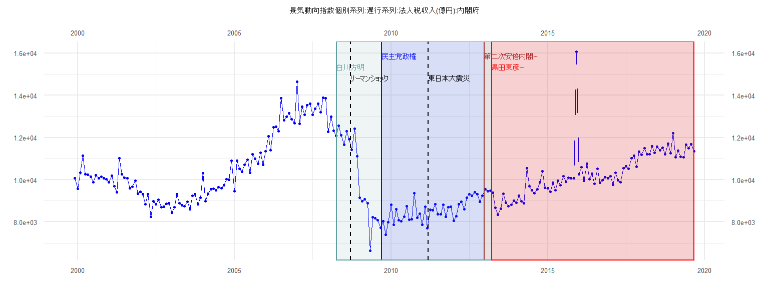
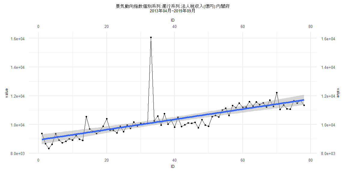
[1] "景気動向指数個別系列:遅行系列:法人税収入(億円):内閣府"
       Jan   Feb   Mar   Apr   May   Jun   Jul   Aug   Sep   Oct   Nov   Dec
1999                                                                   10062
2000  9565 10333 11141 10251 10238 10133  9884 10215 10078 10149 10062 10029
2001  9886 10194  9683  9410 11008 10264 10091 10080  9597  9664  9948  9336
2002  9438  9314  8840  9309  8247  8970  8838  9042  8703  8718  8862  8886
2003  8439  8697  9314  8879  8800  8746  8959  8600  9245  9303  8845  9138
2004 10315  8981  9342  9538  9579  9502  9633  9586  9733 10024 10000 10900
2005  9444 10897 10513 10369 10712 10953 10334 11208 11006 10763 11270 10717
2006 11354 12065 11407 12497 12508 12290 13859 12819 12979 13164 12869 12681
2007 14650 12645 13452 13085 13525 13609 13093 13363 13596 13199 13883 13869
2008 12272 12992 12312 12078 12549 12106 11657 12300 11915 11419 12414 11123
2009  9156  8970  9070  8876  6644  8221  8176  8089  7730  8033  7394  7987
2010  8803  7867  8600  8075  8032  8238  8740  8108  8138  9350  8191  8380
2011  7877  8713  7711  8576  8542  8830  8361  8367  8816  8239  8700  8715
2012  8062  8270  8850  8967  8610  9150  9301  9232  9404  9312  8962  9247
2013  9559  9458  9482  9378  8671  8332  8621  9347  8913  8737  8826  9009
2014  8913  9231  8979  8895 10549  9689  9514  9371  9550  9881 10405  9609
2015  9598  9426  9869  9496  9952  9737 10168  9901 10086 10067 10074 16068
2016 10264 10590  9959 10755 10024 10289  9817 10513  9858  9982 10108 10081
2017 10157  9768 10340  9970  9880 10547 10641 10527 11010 11135 10626 11329
2018 11175 11499 11200 11208 11595 11288 11564 11390 11508 11214 11696 11260
2019 12215 11060 11372 11096 11065 11656 11492 11677 11345
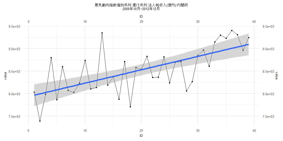
Call:
lm(formula = value ~ ID)

Residuals:
    Min      1Q  Median      3Q     Max
-761.63 -191.08   -3.49  242.98 1025.93

Coefficients:
            Estimate Std. Error t value             Pr(>|t|)
(Intercept) 7937.816    124.252  63.885 < 0.0000000000000002 ***
ID            29.712      5.414   5.488            0.0000031 ***
---
Signif. codes:  0 '***' 0.001 '**' 0.01 '*' 0.05 '.' 0.1 ' ' 1

Residual standard error: 380.5 on 37 degrees of freedom
Multiple R-squared:  0.4487,    Adjusted R-squared:  0.4338
F-statistic: 30.12 on 1 and 37 DF,  p-value: 0.000003102


    Two-sample Kolmogorov-Smirnov test

data:  lm_residuals and rnorm(n = length(lm_residuals), mean = 0, sd = sd(lm_residuals))
D = 0.15385, p-value = 0.7523
alternative hypothesis: two-sided


    Durbin-Watson test

data:  value ~ ID
DW = 2.2181, p-value = 0.6974
alternative hypothesis: true autocorrelation is greater than 0


    studentized Breusch-Pagan test

data:  value ~ ID
BP = 1.1244, df = 1, p-value = 0.289


    Box-Ljung test

data:  lm_residuals
X-squared = 0.52364, df = 1, p-value = 0.4693
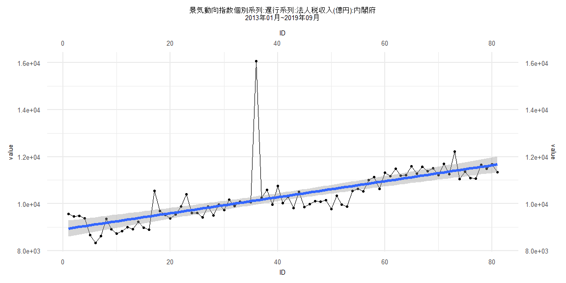
Call:
lm(formula = value ~ ID)

Residuals:
   Min     1Q Median     3Q    Max
-848.6 -372.8  -96.6  162.8 5928.4

Coefficients:
            Estimate Std. Error t value             Pr(>|t|)
(Intercept) 8912.791    173.913  51.249 < 0.0000000000000002 ***
ID            34.077      3.685   9.248   0.0000000000000319 ***
---
Signif. codes:  0 '***' 0.001 '**' 0.01 '*' 0.05 '.' 0.1 ' ' 1

Residual standard error: 775.4 on 79 degrees of freedom
Multiple R-squared:  0.5198,    Adjusted R-squared:  0.5138
F-statistic: 85.53 on 1 and 79 DF,  p-value: 0.0000000000000319


    Two-sample Kolmogorov-Smirnov test

data:  lm_residuals and rnorm(n = length(lm_residuals), mean = 0, sd = sd(lm_residuals))
D = 0.24691, p-value = 0.01405
alternative hypothesis: two-sided


    Durbin-Watson test

data:  value ~ ID
DW = 1.8066, p-value = 0.1608
alternative hypothesis: true autocorrelation is greater than 0


    studentized Breusch-Pagan test

data:  value ~ ID
BP = 0.080485, df = 1, p-value = 0.7766


    Box-Ljung test

data:  lm_residuals
X-squared = 0.70574, df = 1, p-value = 0.4009
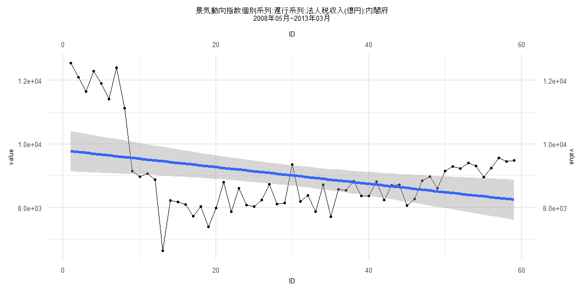
Call:
lm(formula = value ~ ID)

Residuals:
    Min      1Q  Median      3Q     Max
-2814.7  -889.0  -320.2   821.1  2797.4

Coefficients:
            Estimate Std. Error t value             Pr(>|t|)
(Intercept) 9800.793    326.158  30.049 < 0.0000000000000002 ***
ID           -26.318      9.455  -2.784              0.00728 **
---
Signif. codes:  0 '***' 0.001 '**' 0.01 '*' 0.05 '.' 0.1 ' ' 1

Residual standard error: 1237 on 57 degrees of freedom
Multiple R-squared:  0.1197,    Adjusted R-squared:  0.1042
F-statistic: 7.748 on 1 and 57 DF,  p-value: 0.007282


    Two-sample Kolmogorov-Smirnov test

data:  lm_residuals and rnorm(n = length(lm_residuals), mean = 0, sd = sd(lm_residuals))
D = 0.16949, p-value = 0.3674
alternative hypothesis: two-sided


    Durbin-Watson test

data:  value ~ ID
DW = 0.31454, p-value < 0.00000000000000022
alternative hypothesis: true autocorrelation is greater than 0


    studentized Breusch-Pagan test

data:  value ~ ID
BP = 20.313, df = 1, p-value = 0.000006577


    Box-Ljung test

data:  lm_residuals
X-squared = 38.712, df = 1, p-value = 0.0000000004912
Call:
lm(formula = value ~ ID)

Residuals:
   Min     1Q Median     3Q    Max
-840.7 -360.3 -100.8  148.5 5958.8

Coefficients:
            Estimate Std. Error t value             Pr(>|t|)
(Intercept) 8931.965    178.933  49.918 < 0.0000000000000002 ***
ID            35.675      3.936   9.065      0.0000000000001 ***
---
Signif. codes:  0 '***' 0.001 '**' 0.01 '*' 0.05 '.' 0.1 ' ' 1

Residual standard error: 782.6 on 76 degrees of freedom
Multiple R-squared:  0.5195,    Adjusted R-squared:  0.5132
F-statistic: 82.17 on 1 and 76 DF,  p-value: 0.0000000000001003


    Two-sample Kolmogorov-Smirnov test

data:  lm_residuals and rnorm(n = length(lm_residuals), mean = 0, sd = sd(lm_residuals))
D = 0.26923, p-value = 0.006781
alternative hypothesis: two-sided


    Durbin-Watson test

data:  value ~ ID
DW = 1.8428, p-value = 0.2073
alternative hypothesis: true autocorrelation is greater than 0


    studentized Breusch-Pagan test

data:  value ~ ID
BP = 0.10526, df = 1, p-value = 0.7456


    Box-Ljung test

data:  lm_residuals
X-squared = 0.45994, df = 1, p-value = 0.4977