Analysis
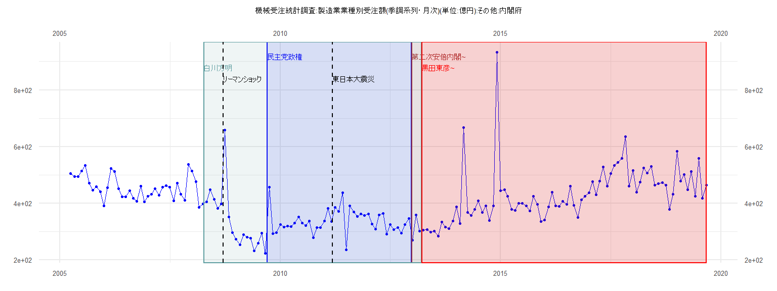
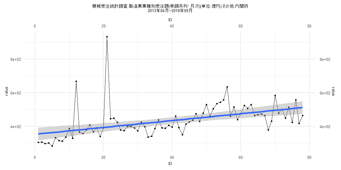
[1] "機械受注統計調査:製造業業種別受注額(季調系列・月次)(単位:億円):その他:内閣府"
        Jan    Feb    Mar    Apr    May    Jun    Jul    Aug    Sep    Oct    Nov    Dec
2005                      505.56 494.20 493.12 513.83 532.64 470.10 445.79 458.30 439.96
2006 390.36 454.79 522.91 511.20 452.00 423.30 423.29 443.35 416.36 406.31 459.34 405.23
2007 424.65 430.85 450.68 428.22 457.01 461.54 457.33 408.43 470.57 431.10 410.63 537.20
2008 513.31 475.39 384.94 396.73 405.00 448.30 413.03 382.03 397.73 658.07 351.52 295.11
2009 272.64 253.18 288.88 280.41 276.62 231.37 258.54 294.99 223.54 456.56 293.22 295.82
2010 325.09 314.75 319.47 317.25 330.42 352.06 330.01 321.73 337.18 277.45 314.15 313.00
2011 337.52 381.05 335.39 385.19 370.87 436.94 235.04 389.89 368.52 352.76 362.77 357.27
2012 361.31 326.17 308.68 358.28 364.04 289.70 325.30 306.42 314.56 293.64 324.41 346.26
2013 269.90 358.16 301.51 305.05 306.74 297.11 301.01 283.34 333.25 315.04 310.50 336.12
2014 386.49 328.74 667.56 366.44 356.30 378.86 408.54 367.08 390.10 338.70 390.09 932.84
2015 444.63 447.61 423.59 377.76 375.10 399.97 399.33 389.87 372.01 424.79 396.50 335.85
2016 341.27 386.17 438.58 391.19 388.85 406.08 396.41 459.90 392.54 350.01 412.61 424.83
2017 436.26 475.38 429.67 478.47 528.23 459.76 503.80 533.58 543.96 557.73 634.25 460.56
2018 515.40 439.14 474.89 523.45 506.15 528.86 463.75 469.87 473.24 463.49 378.57 431.42
2019 583.96 477.82 501.70 447.70 512.71 424.47 557.92 416.97 463.43
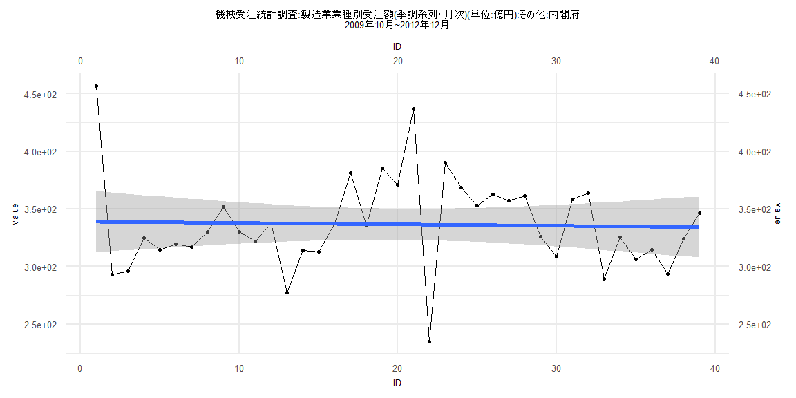
Call:
lm(formula = value ~ ID)

Residuals:
     Min       1Q   Median       3Q      Max
-101.388  -23.493   -7.873   24.276  117.586

Coefficients:
            Estimate Std. Error t value            Pr(>|t|)
(Intercept) 339.0950    13.5695  24.989 <0.0000000000000002 ***
ID           -0.1212     0.5913  -0.205               0.839
---
Signif. codes:  0 '***' 0.001 '**' 0.01 '*' 0.05 '.' 0.1 ' ' 1

Residual standard error: 41.56 on 37 degrees of freedom
Multiple R-squared:  0.001135,  Adjusted R-squared:  -0.02586
F-statistic: 0.04204 on 1 and 37 DF,  p-value: 0.8387


    Two-sample Kolmogorov-Smirnov test

data:  lm_residuals and rnorm(n = length(lm_residuals), mean = 0, sd = sd(lm_residuals))
D = 0.12821, p-value = 0.9114
alternative hypothesis: two-sided


    Durbin-Watson test

data:  value ~ ID
DW = 1.9458, p-value = 0.3657
alternative hypothesis: true autocorrelation is greater than 0


    studentized Breusch-Pagan test

data:  value ~ ID
BP = 1.2896, df = 1, p-value = 0.2561


    Box-Ljung test

data:  lm_residuals
X-squared = 0.2841, df = 1, p-value = 0.594
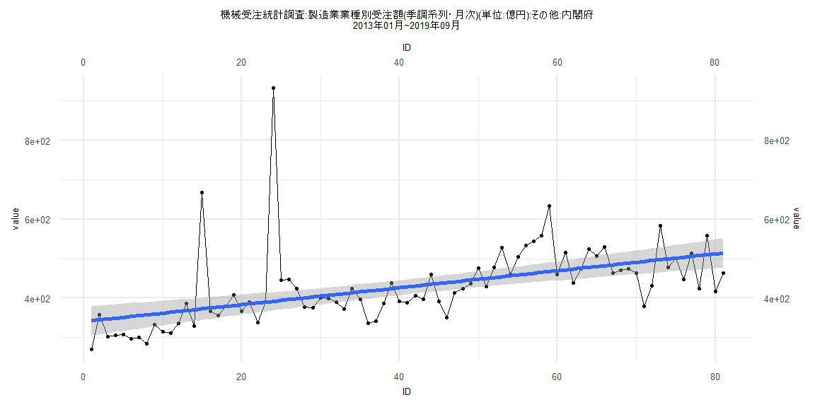
Call:
lm(formula = value ~ ID)

Residuals:
    Min      1Q  Median      3Q     Max
-114.28  -41.68  -18.62   25.04  540.94

Coefficients:
            Estimate Std. Error t value             Pr(>|t|)
(Intercept) 340.3525    19.0963  17.823 < 0.0000000000000002 ***
ID            2.1478     0.4046   5.309          0.000000988 ***
---
Signif. codes:  0 '***' 0.001 '**' 0.01 '*' 0.05 '.' 0.1 ' ' 1

Residual standard error: 85.14 on 79 degrees of freedom
Multiple R-squared:  0.2629,    Adjusted R-squared:  0.2536
F-statistic: 28.18 on 1 and 79 DF,  p-value: 0.0000009876


    Two-sample Kolmogorov-Smirnov test

data:  lm_residuals and rnorm(n = length(lm_residuals), mean = 0, sd = sd(lm_residuals))
D = 0.24691, p-value = 0.01405
alternative hypothesis: two-sided


    Durbin-Watson test

data:  value ~ ID
DW = 1.695, p-value = 0.06662
alternative hypothesis: true autocorrelation is greater than 0


    studentized Breusch-Pagan test

data:  value ~ ID
BP = 0.64725, df = 1, p-value = 0.4211


    Box-Ljung test

data:  lm_residuals
X-squared = 1.7829, df = 1, p-value = 0.1818
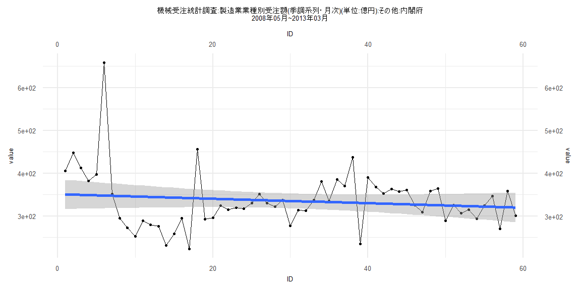
Call:
lm(formula = value ~ ID)

Residuals:
     Min       1Q   Median       3Q      Max
-118.709  -40.054   -6.998   33.943  310.055

Coefficients:
            Estimate Std. Error t value            Pr(>|t|)
(Intercept) 351.1596    17.5069  20.058 <0.0000000000000002 ***
ID           -0.5242     0.5075  -1.033               0.306
---
Signif. codes:  0 '***' 0.001 '**' 0.01 '*' 0.05 '.' 0.1 ' ' 1

Residual standard error: 66.38 on 57 degrees of freedom
Multiple R-squared:  0.01837,   Adjusted R-squared:  0.001149
F-statistic: 1.067 on 1 and 57 DF,  p-value: 0.3061


    Two-sample Kolmogorov-Smirnov test

data:  lm_residuals and rnorm(n = length(lm_residuals), mean = 0, sd = sd(lm_residuals))
D = 0.16949, p-value = 0.3674
alternative hypothesis: two-sided


    Durbin-Watson test

data:  value ~ ID
DW = 1.4974, p-value = 0.0174
alternative hypothesis: true autocorrelation is greater than 0


    studentized Breusch-Pagan test

data:  value ~ ID
BP = 4.8116, df = 1, p-value = 0.02827


    Box-Ljung test

data:  lm_residuals
X-squared = 3.7164, df = 1, p-value = 0.05388
Call:
lm(formula = value ~ ID)

Residuals:
    Min      1Q  Median      3Q     Max
-112.55  -41.45  -19.29   23.19  537.61

Coefficients:
            Estimate Std. Error t value             Pr(>|t|)
(Intercept) 352.3843    19.7066  17.882 < 0.0000000000000002 ***
ID            2.0402     0.4334   4.707            0.0000111 ***
---
Signif. codes:  0 '***' 0.001 '**' 0.01 '*' 0.05 '.' 0.1 ' ' 1

Residual standard error: 86.19 on 76 degrees of freedom
Multiple R-squared:  0.2257,    Adjusted R-squared:  0.2155
F-statistic: 22.16 on 1 and 76 DF,  p-value: 0.00001106


    Two-sample Kolmogorov-Smirnov test

data:  lm_residuals and rnorm(n = length(lm_residuals), mean = 0, sd = sd(lm_residuals))
D = 0.25641, p-value = 0.01157
alternative hypothesis: two-sided


    Durbin-Watson test

data:  value ~ ID
DW = 1.7, p-value = 0.0728
alternative hypothesis: true autocorrelation is greater than 0


    studentized Breusch-Pagan test

data:  value ~ ID
BP = 0.89041, df = 1, p-value = 0.3454


    Box-Ljung test

data:  lm_residuals
X-squared = 1.7222, df = 1, p-value = 0.1894