Analysis
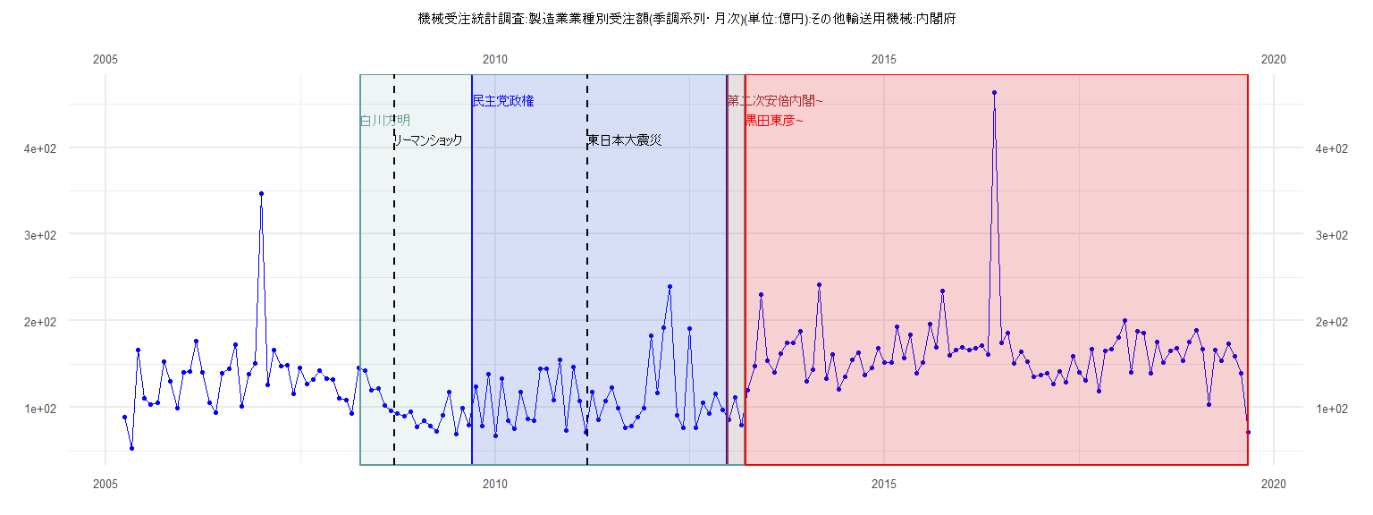
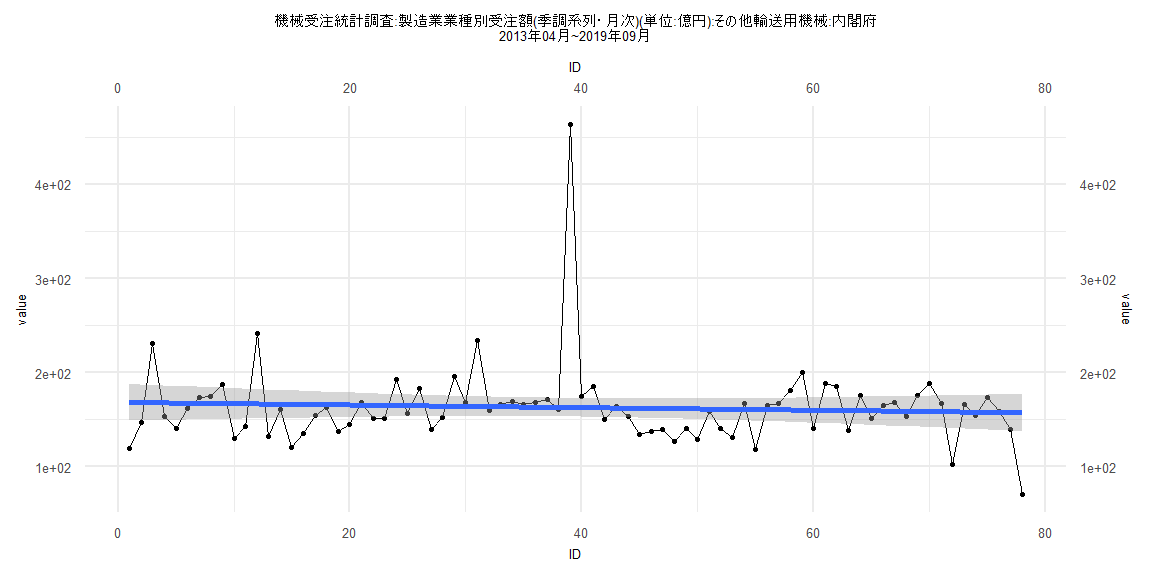
[1] "機械受注統計調査:製造業業種別受注額(季調系列・月次)(単位:億円):その他輸送用機械:内閣府"
        Jan    Feb    Mar    Apr    May    Jun    Jul    Aug    Sep    Oct    Nov    Dec
2005                       89.00  53.20 166.47 110.47 103.36 105.13 152.84 130.28  99.30
2006 140.13 141.04 176.30 140.32 104.94  93.68 139.62 144.26 172.37 101.45 138.08 150.93
2007 347.25 125.78 165.87 147.76 149.20 116.01 145.14 126.71 132.55 143.04 133.44 131.95
2008 110.88 108.64  93.29 145.61 142.84 119.35 122.38 101.81  96.54  93.19  89.41  95.41
2009  77.52  84.56  78.50  72.02  90.54 117.73  69.40  99.45  80.06 124.15  78.10 137.90
2010  67.44 132.90  84.70  75.59 117.91  86.75  84.54 144.51 144.44 108.53 155.00  73.70
2011 146.47 107.26  71.83 117.32  85.78 107.60 122.96  99.21  76.74  78.11  88.54  98.97
2012 183.28 116.62 191.92 239.27  91.44  76.74 190.69  76.62 105.13  92.53 115.35  97.47
2013  86.27 111.22  79.92 119.54 147.29 230.59 153.39 140.97 162.45 174.13 174.75 187.49
2014 130.60 143.16 242.10 132.83 160.89 120.74 135.20 154.95 163.09 137.62 145.38 168.19
2015 151.97 151.60 192.97 156.66 183.50 139.62 152.01 196.54 168.88 233.88 160.25 166.43
2016 169.74 166.71 168.60 171.89 161.01 463.46 174.73 185.56 150.35 164.15 153.09 134.97
2017 137.68 139.59 126.60 141.09 129.54 159.29 140.87 130.76 167.17 118.86 164.85 167.55
2018 181.13 199.91 140.30 188.42 185.42 139.13 175.38 151.47 165.36 168.44 153.44 175.75
2019 189.11 167.16 103.00 166.06 154.24 173.73 159.27 139.59  70.83
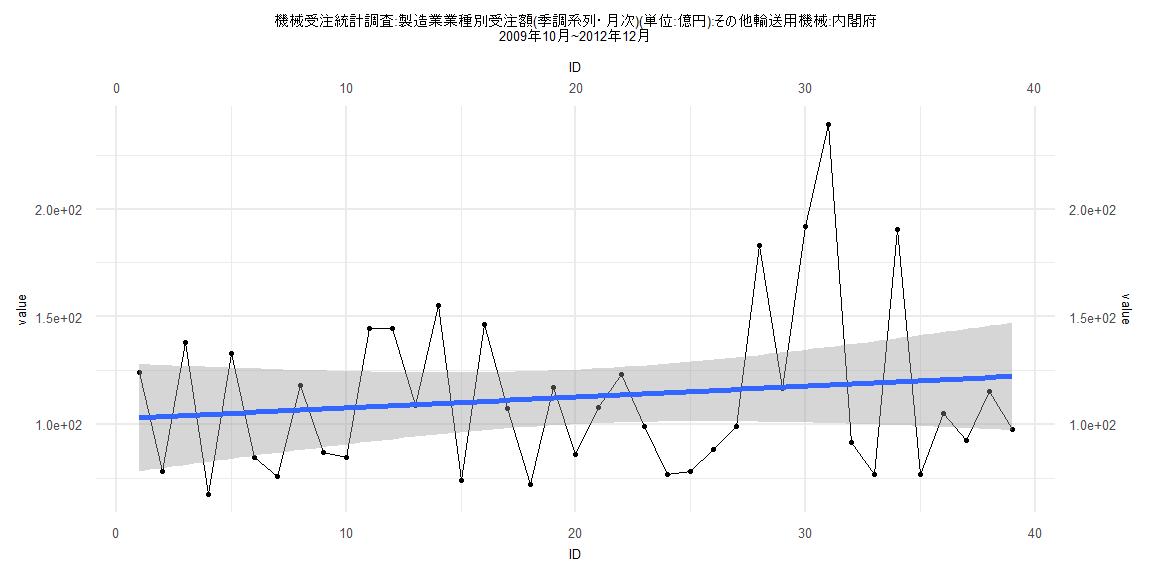
Call:
lm(formula = value ~ ID)

Residuals:
   Min     1Q Median     3Q    Max
-43.61 -27.21 -14.97  24.43 121.06

Coefficients:
            Estimate Std. Error t value      Pr(>|t|)
(Intercept) 102.5885    12.7541   8.044 0.00000000121 ***
ID            0.5039     0.5558   0.907          0.37
---
Signif. codes:  0 '***' 0.001 '**' 0.01 '*' 0.05 '.' 0.1 ' ' 1

Residual standard error: 39.06 on 37 degrees of freedom
Multiple R-squared:  0.02174,   Adjusted R-squared:  -0.004702
F-statistic: 0.8222 on 1 and 37 DF,  p-value: 0.3704


    Two-sample Kolmogorov-Smirnov test

data:  lm_residuals and rnorm(n = length(lm_residuals), mean = 0, sd = sd(lm_residuals))
D = 0.20513, p-value = 0.3888
alternative hypothesis: two-sided


    Durbin-Watson test

data:  value ~ ID
DW = 2.0602, p-value = 0.5069
alternative hypothesis: true autocorrelation is greater than 0


    studentized Breusch-Pagan test

data:  value ~ ID
BP = 2.5805, df = 1, p-value = 0.1082


    Box-Ljung test

data:  lm_residuals
X-squared = 0.065537, df = 1, p-value = 0.7979
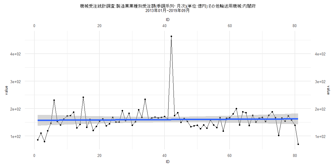
Call:
lm(formula = value ~ ID)

Residuals:
    Min      1Q  Median      3Q     Max
-92.054 -21.368  -1.917  11.032 302.999

Coefficients:
             Estimate Std. Error t value            Pr(>|t|)
(Intercept) 157.85201   10.13949  15.568 <0.0000000000000002 ***
ID            0.06212    0.21483   0.289               0.773
---
Signif. codes:  0 '***' 0.001 '**' 0.01 '*' 0.05 '.' 0.1 ' ' 1

Residual standard error: 45.21 on 79 degrees of freedom
Multiple R-squared:  0.001057,  Adjusted R-squared:  -0.01159
F-statistic: 0.08362 on 1 and 79 DF,  p-value: 0.7732


    Two-sample Kolmogorov-Smirnov test

data:  lm_residuals and rnorm(n = length(lm_residuals), mean = 0, sd = sd(lm_residuals))
D = 0.23457, p-value = 0.02289
alternative hypothesis: two-sided


    Durbin-Watson test

data:  value ~ ID
DW = 1.7114, p-value = 0.07694
alternative hypothesis: true autocorrelation is greater than 0


    studentized Breusch-Pagan test

data:  value ~ ID
BP = 0.030775, df = 1, p-value = 0.8607


    Box-Ljung test

data:  lm_residuals
X-squared = 0.87717, df = 1, p-value = 0.349
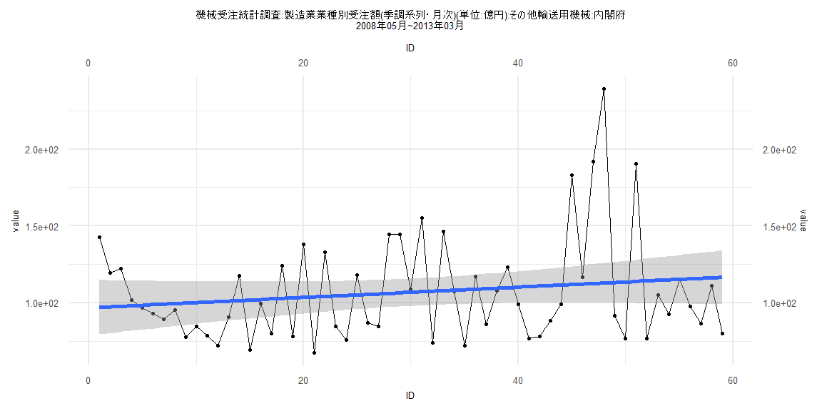
Call:
lm(formula = value ~ ID)

Residuals:
    Min      1Q  Median      3Q     Max
-37.607 -22.516  -9.434  14.708 126.391

Coefficients:
            Estimate Std. Error t value            Pr(>|t|)
(Intercept)  96.7100     9.0169  10.725 0.00000000000000271 ***
ID            0.3369     0.2614   1.289               0.203
---
Signif. codes:  0 '***' 0.001 '**' 0.01 '*' 0.05 '.' 0.1 ' ' 1

Residual standard error: 34.19 on 57 degrees of freedom
Multiple R-squared:  0.02831,   Adjusted R-squared:  0.01127
F-statistic: 1.661 on 1 and 57 DF,  p-value: 0.2027


    Two-sample Kolmogorov-Smirnov test

data:  lm_residuals and rnorm(n = length(lm_residuals), mean = 0, sd = sd(lm_residuals))
D = 0.20339, p-value = 0.1748
alternative hypothesis: two-sided


    Durbin-Watson test

data:  value ~ ID
DW = 1.8941, p-value = 0.2925
alternative hypothesis: true autocorrelation is greater than 0


    studentized Breusch-Pagan test

data:  value ~ ID
BP = 3.7037, df = 1, p-value = 0.05429


    Box-Ljung test

data:  lm_residuals
X-squared = 0.045696, df = 1, p-value = 0.8307
Call:
lm(formula = value ~ ID)

Residuals:
    Min      1Q  Median      3Q     Max
-86.830 -20.612  -3.357   8.530 300.379

Coefficients:
            Estimate Std. Error t value            Pr(>|t|)
(Intercept) 168.5024    10.0192  16.818 <0.0000000000000002 ***
ID           -0.1390     0.2204  -0.631                0.53
---
Signif. codes:  0 '***' 0.001 '**' 0.01 '*' 0.05 '.' 0.1 ' ' 1

Residual standard error: 43.82 on 76 degrees of freedom
Multiple R-squared:  0.005208,  Adjusted R-squared:  -0.007881
F-statistic: 0.3979 on 1 and 76 DF,  p-value: 0.5301


    Two-sample Kolmogorov-Smirnov test

data:  lm_residuals and rnorm(n = length(lm_residuals), mean = 0, sd = sd(lm_residuals))
D = 0.15385, p-value = 0.316
alternative hypothesis: two-sided


    Durbin-Watson test

data:  value ~ ID
DW = 1.8715, p-value = 0.2458
alternative hypothesis: true autocorrelation is greater than 0


    studentized Breusch-Pagan test

data:  value ~ ID
BP = 0.004573, df = 1, p-value = 0.9461


    Box-Ljung test

data:  lm_residuals
X-squared = 0.0741, df = 1, p-value = 0.7855