Analysis
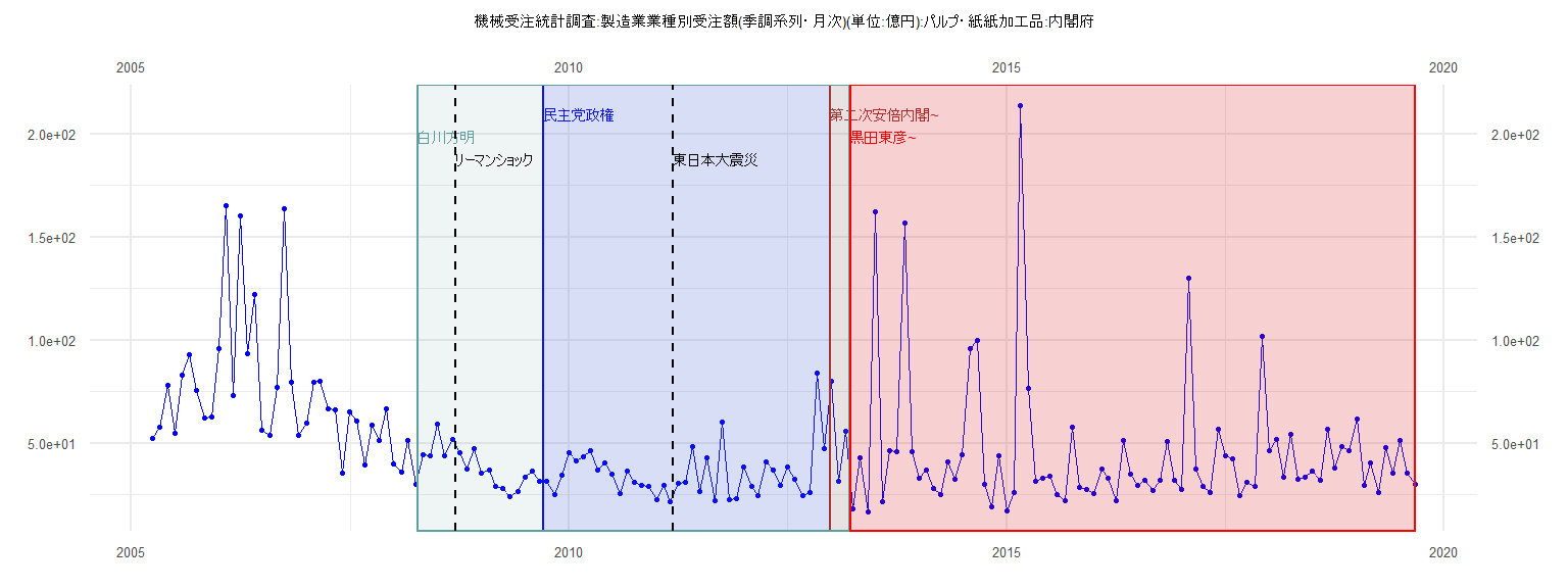
[1] "機械受注統計調査:製造業業種別受注額(季調系列・月次)(単位:億円):パルプ・紙紙加工品:内閣府"
        Jan    Feb    Mar    Apr    May    Jun    Jul    Aug    Sep    Oct    Nov    Dec
2005                       52.18  57.62  78.10  54.71  83.23  92.94  75.77  62.11  62.84
2006  95.87 165.28  73.20 160.16  93.42 122.23  56.52  53.60  77.02 163.68  79.75  53.87
2007  59.78  79.37  80.13  66.73  66.24  35.56  65.26  60.58  39.61  58.99  51.50  66.64
2008  39.89  35.80  51.51  30.21  44.61  43.80  59.41  43.96  52.03  45.45  37.51  47.41
2009  35.35  36.83  29.24  28.11  23.92  26.81  33.60  36.55  31.45  31.56  25.33  34.49
2010  45.54  41.35  43.56  46.36  37.22  40.60  35.00  25.39  36.74  31.14  29.57  28.95
2011  22.59  29.62  21.43  30.52  30.86  48.53  26.79  43.07  22.40  60.48  22.56  23.32
2012  38.45  28.99  24.59  40.99  37.16  29.37  38.65  32.47  24.80  26.00  83.98  47.34
2013  80.11  31.79  55.58  18.35  42.75  16.94 162.41  21.59  46.31  45.87 156.62  46.04
2014  33.19  37.16  28.33  24.91  41.10  32.31  44.30  95.95  99.70  30.28  19.43  43.99
2015  17.25  26.15 213.59  76.76  31.50  32.91  34.12  25.06  22.05  58.00  28.52  27.69
2016  25.55  37.29  33.11  21.99  51.31  35.22  29.62  31.91  27.28  31.94  50.82  32.23
2017  27.47 129.87  37.36  28.89  26.02  56.89  43.93  42.25  24.42  31.00  29.03 101.80
2018  46.24  51.67  33.30  54.43  32.43  33.43  36.74  32.24  56.62  37.79  48.26  46.35
2019  61.55  29.39  40.31  26.23  47.92  35.61  51.50  35.32  29.99
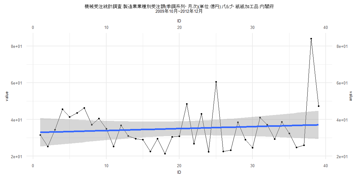
Call:
lm(formula = value ~ ID)

Residuals:
    Min      1Q  Median      3Q     Max
-13.426  -8.150  -3.178   5.724  46.973

Coefficients:
            Estimate Std. Error t value       Pr(>|t|)
(Intercept)  32.9199     3.9513   8.331 0.000000000518 ***
ID            0.1075     0.1722   0.625          0.536
---
Signif. codes:  0 '***' 0.001 '**' 0.01 '*' 0.05 '.' 0.1 ' ' 1

Residual standard error: 12.1 on 37 degrees of freedom
Multiple R-squared:  0.01043,   Adjusted R-squared:  -0.01631
F-statistic: 0.3901 on 1 and 37 DF,  p-value: 0.5361


    Two-sample Kolmogorov-Smirnov test

data:  lm_residuals and rnorm(n = length(lm_residuals), mean = 0, sd = sd(lm_residuals))
D = 0.20513, p-value = 0.3888
alternative hypothesis: two-sided


    Durbin-Watson test

data:  value ~ ID
DW = 1.9987, p-value = 0.43
alternative hypothesis: true autocorrelation is greater than 0


    studentized Breusch-Pagan test

data:  value ~ ID
BP = 3.2781, df = 1, p-value = 0.07021


    Box-Ljung test

data:  lm_residuals
X-squared = 0.0035793, df = 1, p-value = 0.9523
Call:
lm(formula = value ~ ID)

Residuals:
    Min      1Q  Median      3Q     Max
-35.753 -17.306  -8.504   5.592 165.082

Coefficients:
            Estimate Std. Error t value       Pr(>|t|)
(Intercept)  53.8890     7.3711   7.311 0.000000000189 ***
ID           -0.1993     0.1562  -1.276          0.206
---
Signif. codes:  0 '***' 0.001 '**' 0.01 '*' 0.05 '.' 0.1 ' ' 1

Residual standard error: 32.86 on 79 degrees of freedom
Multiple R-squared:  0.0202,    Adjusted R-squared:  0.007796
F-statistic: 1.629 on 1 and 79 DF,  p-value: 0.2056


    Two-sample Kolmogorov-Smirnov test

data:  lm_residuals and rnorm(n = length(lm_residuals), mean = 0, sd = sd(lm_residuals))
D = 0.19753, p-value = 0.08471
alternative hypothesis: two-sided


    Durbin-Watson test

data:  value ~ ID
DW = 2.0616, p-value = 0.5649
alternative hypothesis: true autocorrelation is greater than 0


    studentized Breusch-Pagan test

data:  value ~ ID
BP = 3.0884, df = 1, p-value = 0.07885


    Box-Ljung test

data:  lm_residuals
X-squared = 0.10451, df = 1, p-value = 0.7465
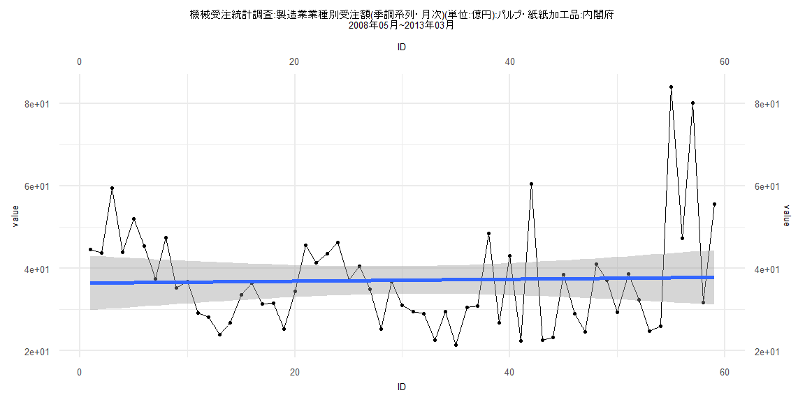
Call:
lm(formula = value ~ ID)

Residuals:
    Min      1Q  Median      3Q     Max
-15.829  -8.387  -2.069   6.954  46.247

Coefficients:
            Estimate Std. Error t value            Pr(>|t|)
(Intercept) 36.42947    3.37966  10.779 0.00000000000000224 ***
ID           0.02370    0.09797   0.242                0.81
---
Signif. codes:  0 '***' 0.001 '**' 0.01 '*' 0.05 '.' 0.1 ' ' 1

Residual standard error: 12.82 on 57 degrees of freedom
Multiple R-squared:  0.001025,  Adjusted R-squared:  -0.0165
F-statistic: 0.0585 on 1 and 57 DF,  p-value: 0.8098


    Two-sample Kolmogorov-Smirnov test

data:  lm_residuals and rnorm(n = length(lm_residuals), mean = 0, sd = sd(lm_residuals))
D = 0.15254, p-value = 0.5021
alternative hypothesis: two-sided


    Durbin-Watson test

data:  value ~ ID
DW = 1.6956, p-value = 0.09352
alternative hypothesis: true autocorrelation is greater than 0


    studentized Breusch-Pagan test

data:  value ~ ID
BP = 5.2199, df = 1, p-value = 0.02233


    Box-Ljung test

data:  lm_residuals
X-squared = 1.0777, df = 1, p-value = 0.2992
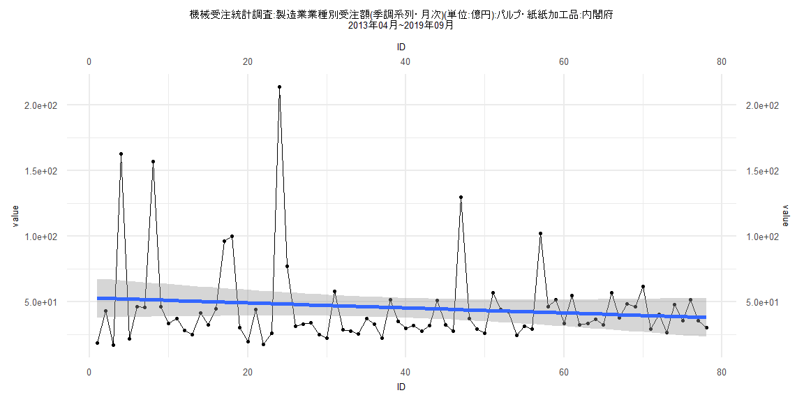
Call:
lm(formula = value ~ ID)

Residuals:
    Min      1Q  Median      3Q     Max
-35.379 -17.127  -8.745   5.384 165.293

Coefficients:
            Estimate Std. Error t value      Pr(>|t|)
(Intercept)  52.8935     7.6081   6.952 0.00000000108 ***
ID           -0.1915     0.1673  -1.144         0.256
---
Signif. codes:  0 '***' 0.001 '**' 0.01 '*' 0.05 '.' 0.1 ' ' 1

Residual standard error: 33.27 on 76 degrees of freedom
Multiple R-squared:  0.01694,   Adjusted R-squared:  0.004008
F-statistic:  1.31 on 1 and 76 DF,  p-value: 0.256


    Two-sample Kolmogorov-Smirnov test

data:  lm_residuals and rnorm(n = length(lm_residuals), mean = 0, sd = sd(lm_residuals))
D = 0.24359, p-value = 0.01923
alternative hypothesis: two-sided


    Durbin-Watson test

data:  value ~ ID
DW = 2.0398, p-value = 0.5236
alternative hypothesis: true autocorrelation is greater than 0


    studentized Breusch-Pagan test

data:  value ~ ID
BP = 3.7347, df = 1, p-value = 0.05329


    Box-Ljung test

data:  lm_residuals
X-squared = 0.060408, df = 1, p-value = 0.8059