Analysis
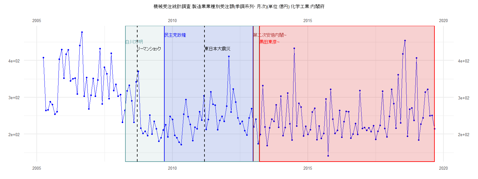
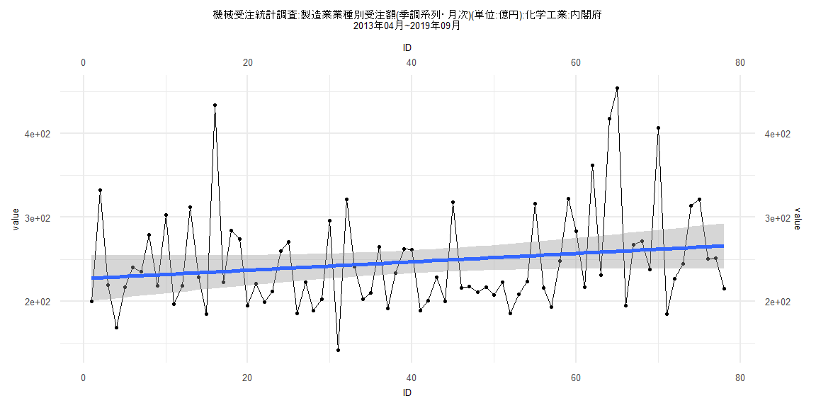
[1] "機械受注統計調査:製造業業種別受注額(季調系列・月次)(単位:億円):化学工業:内閣府"
        Jan    Feb    Mar    Apr    May    Jun    Jul    Aug    Sep    Oct    Nov    Dec
2005                      407.81 264.37 266.36 288.19 280.26 254.33 261.23 403.30 429.92
2006 351.90 417.44 429.17 344.88 350.27 351.94 308.98 440.72 476.86 303.54 353.59 268.73
2007 305.36 351.65 302.97 347.14 432.62 282.54 381.44 364.24 296.47 419.43 318.13 335.44
2008 303.20 307.60 232.09 264.54 317.69 332.96 290.18 232.50 342.32 370.28 216.19 202.44
2009 207.55 196.38 251.69 200.37 234.60 214.72 181.27 190.11 211.69 225.41 192.52 248.33
2010 240.29 196.64 190.58 178.55 171.52 254.22 293.77 247.40 226.32 182.57 219.24 214.81
2011 260.79 238.25 304.35 213.09 239.96 315.33 281.25 278.57 211.80 237.85 248.07 235.00
2012 276.01 410.92 260.07 322.83 286.97 244.61 228.08 234.57 209.31 198.21 243.95 269.90
2013 219.33 240.93 174.31 199.86 332.26 219.48 169.07 217.11 240.71 235.10 279.27 218.80
2014 302.99 196.38 218.33 312.00 228.34 184.67 433.38 222.44 284.08 273.88 194.96 221.08
2015 199.12 212.08 260.21 270.75 185.58 222.50 188.65 202.15 295.92 141.70 321.52 241.10
2016 202.26 210.21 264.55 191.75 234.05 262.27 261.46 189.24 200.60 228.70 199.80 318.17
2017 215.94 217.80 210.51 217.16 207.48 222.70 185.74 208.12 223.63 316.61 215.93 192.97
2018 248.21 322.06 283.16 216.78 361.72 231.05 417.86 453.84 194.61 267.74 271.30 237.83
2019 406.92 184.45 227.07 244.20 313.79 321.67 250.48 250.99 214.90
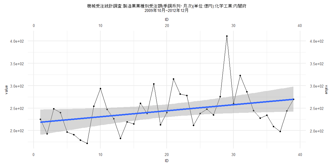
Call:
lm(formula = value ~ ID)

Residuals:
    Min      1Q  Median      3Q     Max
-69.202 -28.748  -4.457  23.246 154.334

Coefficients:
            Estimate Std. Error t value            Pr(>|t|)
(Intercept) 217.3448    14.4081  15.085 <0.0000000000000002 ***
ID            1.3532     0.6278   2.155              0.0377 *
---
Signif. codes:  0 '***' 0.001 '**' 0.01 '*' 0.05 '.' 0.1 ' ' 1

Residual standard error: 44.13 on 37 degrees of freedom
Multiple R-squared:  0.1115,    Adjusted R-squared:  0.08753
F-statistic: 4.645 on 1 and 37 DF,  p-value: 0.03771


    Two-sample Kolmogorov-Smirnov test

data:  lm_residuals and rnorm(n = length(lm_residuals), mean = 0, sd = sd(lm_residuals))
D = 0.30769, p-value = 0.04927
alternative hypothesis: two-sided


    Durbin-Watson test

data:  value ~ ID
DW = 1.4217, p-value = 0.0208
alternative hypothesis: true autocorrelation is greater than 0


    studentized Breusch-Pagan test

data:  value ~ ID
BP = 0.9068, df = 1, p-value = 0.341


    Box-Ljung test

data:  lm_residuals
X-squared = 3.5108, df = 1, p-value = 0.06097
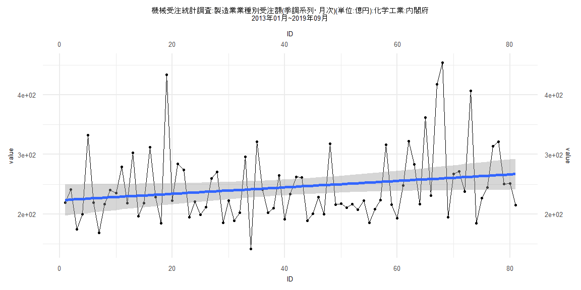
Call:
lm(formula = value ~ ID)

Residuals:
   Min     1Q Median     3Q    Max
-99.94 -40.29 -15.42  22.35 199.83

Coefficients:
            Estimate Std. Error t value            Pr(>|t|)
(Intercept) 223.3040    13.3629  16.711 <0.0000000000000002 ***
ID            0.5392     0.2831   1.904              0.0605 .
---
Signif. codes:  0 '***' 0.001 '**' 0.01 '*' 0.05 '.' 0.1 ' ' 1

Residual standard error: 59.58 on 79 degrees of freedom
Multiple R-squared:  0.0439,    Adjusted R-squared:  0.03179
F-statistic: 3.627 on 1 and 79 DF,  p-value: 0.06049


    Two-sample Kolmogorov-Smirnov test

data:  lm_residuals and rnorm(n = length(lm_residuals), mean = 0, sd = sd(lm_residuals))
D = 0.22222, p-value = 0.03633
alternative hypothesis: two-sided


    Durbin-Watson test

data:  value ~ ID
DW = 2.1562, p-value = 0.7228
alternative hypothesis: true autocorrelation is greater than 0


    studentized Breusch-Pagan test

data:  value ~ ID
BP = 1.0825, df = 1, p-value = 0.2981


    Box-Ljung test

data:  lm_residuals
X-squared = 0.57837, df = 1, p-value = 0.447
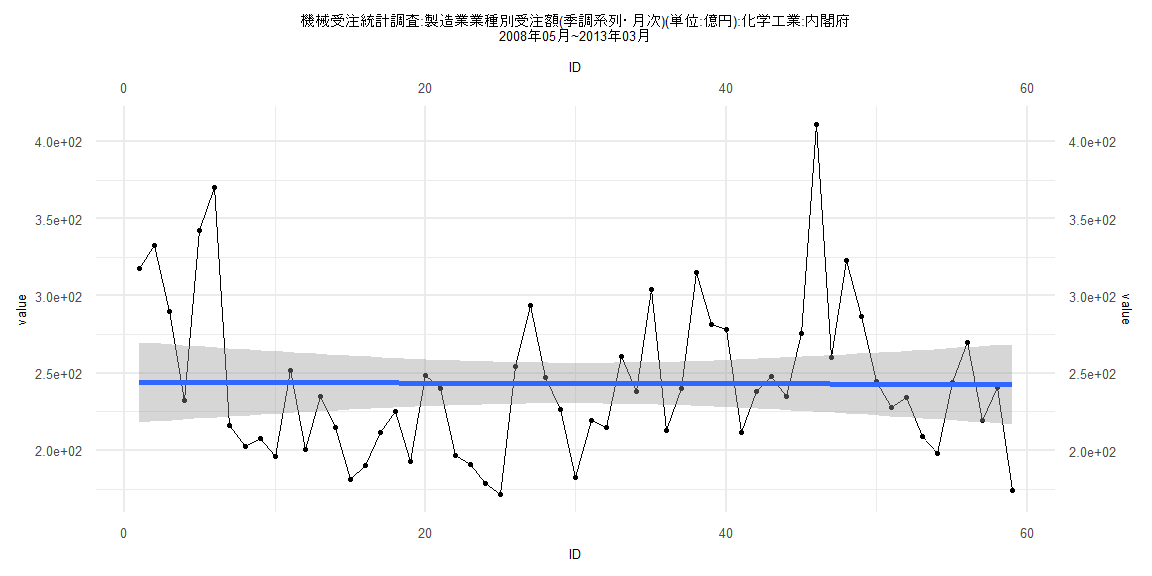
Call:
lm(formula = value ~ ID)

Residuals:
    Min      1Q  Median      3Q     Max
-71.973 -32.767  -8.063  22.293 167.902

Coefficients:
             Estimate Std. Error t value            Pr(>|t|)
(Intercept) 244.05822   13.28534  18.370 <0.0000000000000002 ***
ID           -0.02261    0.38512  -0.059               0.953
---
Signif. codes:  0 '***' 0.001 '**' 0.01 '*' 0.05 '.' 0.1 ' ' 1

Residual standard error: 50.38 on 57 degrees of freedom
Multiple R-squared:  6.045e-05, Adjusted R-squared:  -0.01748
F-statistic: 0.003446 on 1 and 57 DF,  p-value: 0.9534


    Two-sample Kolmogorov-Smirnov test

data:  lm_residuals and rnorm(n = length(lm_residuals), mean = 0, sd = sd(lm_residuals))
D = 0.16949, p-value = 0.3674
alternative hypothesis: two-sided


    Durbin-Watson test

data:  value ~ ID
DW = 1.1155, p-value = 0.00009041
alternative hypothesis: true autocorrelation is greater than 0


    studentized Breusch-Pagan test

data:  value ~ ID
BP = 0.7765, df = 1, p-value = 0.3782


    Box-Ljung test

data:  lm_residuals
X-squared = 10.295, df = 1, p-value = 0.001334
Call:
lm(formula = value ~ ID)

Residuals:
    Min      1Q  Median      3Q     Max
-100.76  -40.17  -15.49   24.95  198.44

Coefficients:
            Estimate Std. Error t value            Pr(>|t|)
(Intercept) 226.9309    13.8157  16.426 <0.0000000000000002 ***
ID            0.5009     0.3039   1.648               0.103
---
Signif. codes:  0 '***' 0.001 '**' 0.01 '*' 0.05 '.' 0.1 ' ' 1

Residual standard error: 60.42 on 76 degrees of freedom
Multiple R-squared:  0.03451,   Adjusted R-squared:  0.02181
F-statistic: 2.717 on 1 and 76 DF,  p-value: 0.1034


    Two-sample Kolmogorov-Smirnov test

data:  lm_residuals and rnorm(n = length(lm_residuals), mean = 0, sd = sd(lm_residuals))
D = 0.15385, p-value = 0.316
alternative hypothesis: two-sided


    Durbin-Watson test

data:  value ~ ID
DW = 2.1589, p-value = 0.7217
alternative hypothesis: true autocorrelation is greater than 0


    studentized Breusch-Pagan test

data:  value ~ ID
BP = 0.78667, df = 1, p-value = 0.3751


    Box-Ljung test

data:  lm_residuals
X-squared = 0.59242, df = 1, p-value = 0.4415