Analysis
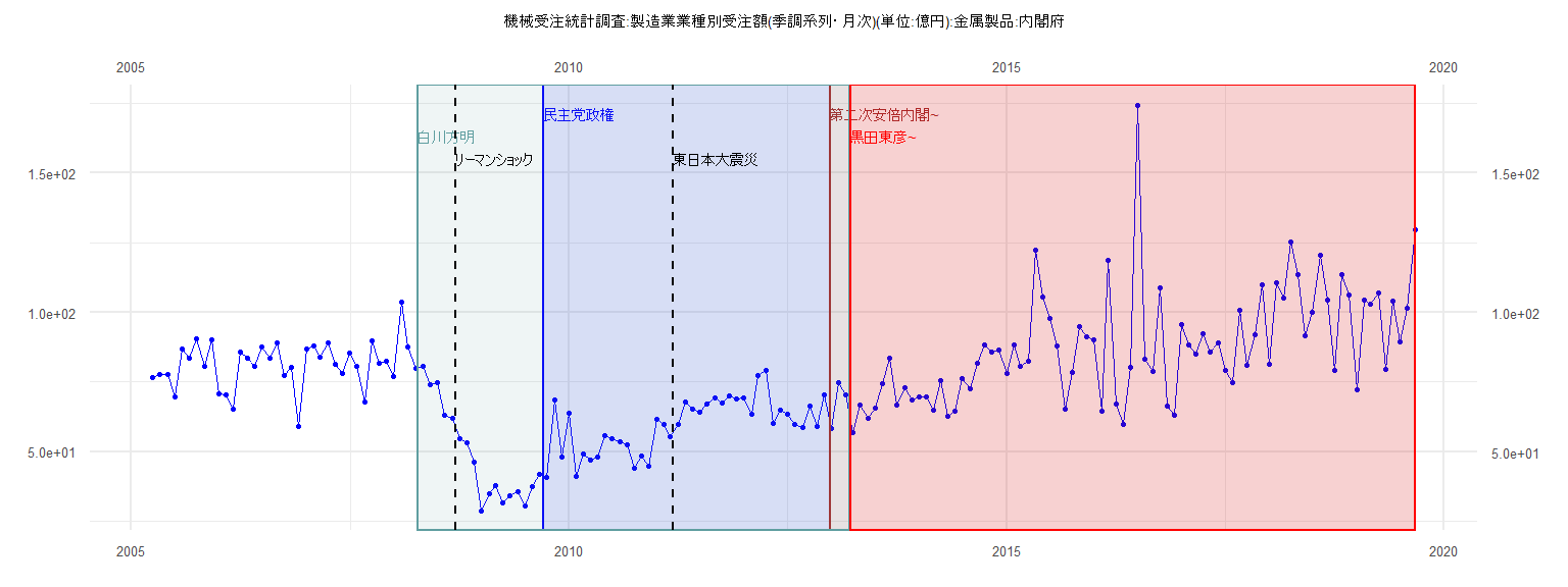
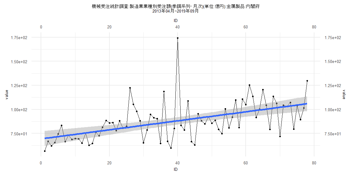
[1] "機械受注統計調査:製造業業種別受注額(季調系列・月次)(単位:億円):金属製品:内閣府"
        Jan    Feb    Mar    Apr    May    Jun    Jul    Aug    Sep    Oct    Nov    Dec
2005                       76.69  77.75  77.78  69.72  86.69  83.48  90.42  80.63  90.07
2006  70.62  70.24  65.21  85.92  83.40  80.74  87.71  83.38  89.19  77.47  80.22  58.96
2007  86.83  87.94  83.98  89.17  81.19  78.02  85.36  80.59  67.68  89.87  81.67  82.32
2008  77.01 103.60  87.68  80.05  80.65  74.07  74.78  62.91  62.08  54.65  53.11  46.11
2009  28.87  34.90  37.83  31.49  34.18  35.65  30.37  37.63  41.74  40.66  68.42  48.20
2010  63.86  41.16  49.23  47.17  48.24  55.60  54.60  53.51  52.49  44.15  48.43  44.85
2011  61.64  59.80  55.24  59.62  67.79  65.28  64.31  67.03  69.33  67.59  69.88  68.97
2012  69.35  63.48  77.38  79.23  60.28  64.75  63.45  59.77  58.56  66.35  59.02  70.48
2013  58.20  74.88  70.26  56.70  66.91  62.03  65.54  74.52  83.42  66.61  73.12  68.68
2014  69.61  69.51  64.83  75.58  62.74  64.47  76.33  72.56  81.61  88.36  85.90  86.33
2015  77.92  88.27  80.52  82.41 122.42 105.31  97.85  88.06  65.10  78.59  94.83  91.25
2016  90.28  64.56 118.70  66.93  59.76  80.32 174.20  83.29  78.72 108.76  66.45  62.97
2017  95.53  88.13  85.02  92.20  85.64  88.87  79.15  74.81 100.58  80.87  92.09 109.72
2018  81.18 110.72 104.94 125.25 113.54  91.53 100.16 120.53 104.22  79.32 113.67 106.31
2019  72.08 104.38 103.09 107.06  79.41 104.06  89.56 101.52 129.79
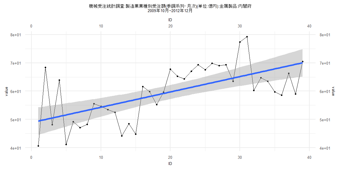
Call:
lm(formula = value ~ ID)

Residuals:
    Min      1Q  Median      3Q     Max
-12.162  -5.243  -1.119   5.226  18.453

Coefficients:
            Estimate Std. Error t value             Pr(>|t|)
(Intercept)  48.8833     2.4859  19.664 < 0.0000000000000002 ***
ID            0.5419     0.1083   5.003             0.000014 ***
---
Signif. codes:  0 '***' 0.001 '**' 0.01 '*' 0.05 '.' 0.1 ' ' 1

Residual standard error: 7.614 on 37 degrees of freedom
Multiple R-squared:  0.4035,    Adjusted R-squared:  0.3874
F-statistic: 25.03 on 1 and 37 DF,  p-value: 0.00001398


    Two-sample Kolmogorov-Smirnov test

data:  lm_residuals and rnorm(n = length(lm_residuals), mean = 0, sd = sd(lm_residuals))
D = 0.17949, p-value = 0.5622
alternative hypothesis: two-sided


    Durbin-Watson test

data:  value ~ ID
DW = 1.6045, p-value = 0.076
alternative hypothesis: true autocorrelation is greater than 0


    studentized Breusch-Pagan test

data:  value ~ ID
BP = 1.0636, df = 1, p-value = 0.3024


    Box-Ljung test

data:  lm_residuals
X-squared = 1.3602, df = 1, p-value = 0.2435
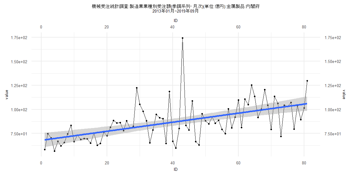
Call:
lm(formula = value ~ ID)

Residuals:
    Min      1Q  Median      3Q     Max
-30.194  -8.628  -0.463   6.435  86.082

Coefficients:
            Estimate Std. Error t value             Pr(>|t|)
(Intercept) 67.82692    3.78179  17.935 < 0.0000000000000002 ***
ID           0.47188    0.08013   5.889           0.00000009 ***
---
Signif. codes:  0 '***' 0.001 '**' 0.01 '*' 0.05 '.' 0.1 ' ' 1

Residual standard error: 16.86 on 79 degrees of freedom
Multiple R-squared:  0.3051,    Adjusted R-squared:  0.2963
F-statistic: 34.68 on 1 and 79 DF,  p-value: 0.00000009001


    Two-sample Kolmogorov-Smirnov test

data:  lm_residuals and rnorm(n = length(lm_residuals), mean = 0, sd = sd(lm_residuals))
D = 0.20988, p-value = 0.05619
alternative hypothesis: two-sided


    Durbin-Watson test

data:  value ~ ID
DW = 1.9792, p-value = 0.4172
alternative hypothesis: true autocorrelation is greater than 0


    studentized Breusch-Pagan test

data:  value ~ ID
BP = 0.43118, df = 1, p-value = 0.5114


    Box-Ljung test

data:  lm_residuals
X-squared = 0.0016524, df = 1, p-value = 0.9676
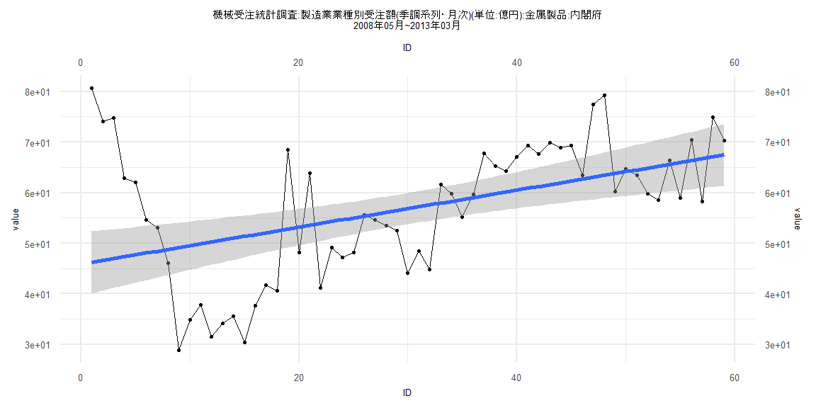
Call:
lm(formula = value ~ ID)

Residuals:
    Min      1Q  Median      3Q     Max
-20.987  -7.992   0.223   6.798  34.410

Coefficients:
            Estimate Std. Error t value             Pr(>|t|)
(Intercept) 45.87477    3.13466  14.635 < 0.0000000000000002 ***
ID           0.36548    0.09087   4.022             0.000172 ***
---
Signif. codes:  0 '***' 0.001 '**' 0.01 '*' 0.05 '.' 0.1 ' ' 1

Residual standard error: 11.89 on 57 degrees of freedom
Multiple R-squared:  0.2211,    Adjusted R-squared:  0.2074
F-statistic: 16.18 on 1 and 57 DF,  p-value: 0.0001717


    Two-sample Kolmogorov-Smirnov test

data:  lm_residuals and rnorm(n = length(lm_residuals), mean = 0, sd = sd(lm_residuals))
D = 0.084746, p-value = 0.9854
alternative hypothesis: two-sided


    Durbin-Watson test

data:  value ~ ID
DW = 0.58493, p-value = 0.00000000002187
alternative hypothesis: true autocorrelation is greater than 0


    studentized Breusch-Pagan test

data:  value ~ ID
BP = 18.071, df = 1, p-value = 0.00002129


    Box-Ljung test

data:  lm_residuals
X-squared = 24.905, df = 1, p-value = 0.0000006024
Call:
lm(formula = value ~ ID)

Residuals:
    Min      1Q  Median      3Q     Max
-30.131  -8.441  -0.536   6.903  86.046

Coefficients:
            Estimate Std. Error t value             Pr(>|t|)
(Intercept) 69.41202    3.91822  17.715 < 0.0000000000000002 ***
ID           0.46856    0.08618   5.437          0.000000632 ***
---
Signif. codes:  0 '***' 0.001 '**' 0.01 '*' 0.05 '.' 0.1 ' ' 1

Residual standard error: 17.14 on 76 degrees of freedom
Multiple R-squared:   0.28, Adjusted R-squared:  0.2706
F-statistic: 29.56 on 1 and 76 DF,  p-value: 0.0000006323


    Two-sample Kolmogorov-Smirnov test

data:  lm_residuals and rnorm(n = length(lm_residuals), mean = 0, sd = sd(lm_residuals))
D = 0.15385, p-value = 0.316
alternative hypothesis: two-sided


    Durbin-Watson test

data:  value ~ ID
DW = 1.97, p-value = 0.4011
alternative hypothesis: true autocorrelation is greater than 0


    studentized Breusch-Pagan test

data:  value ~ ID
BP = 0.26854, df = 1, p-value = 0.6043


    Box-Ljung test

data:  lm_residuals
X-squared = 0.00020913, df = 1, p-value = 0.9885