Analysis
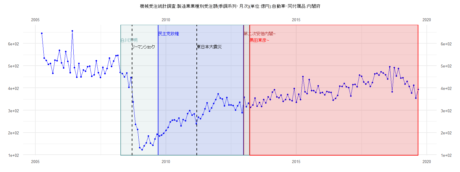
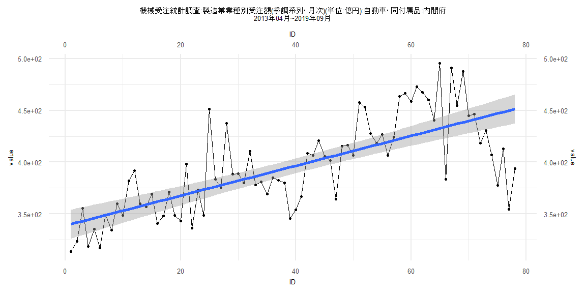
[1] "機械受注統計調査:製造業業種別受注額(季調系列・月次)(単位:億円):自動車・同付属品:内閣府"
        Jan    Feb    Mar    Apr    May    Jun    Jul    Aug    Sep    Oct    Nov    Dec
2005                      645.66 534.52 523.98 506.77 510.54 465.70 525.39 522.84 569.49
2006 513.05 490.32 564.78 519.35 469.57 656.49 492.01 448.32 511.11 450.01 481.04 475.25
2007 495.36 497.97 453.02 459.22 522.72 468.71 448.22 493.41 464.84 487.51 535.26 497.76
2008 520.82 545.22 546.71 469.91 465.61 449.87 467.64 403.13 447.93 338.26 237.74 214.11
2009 133.35 123.92 141.25 154.65 185.51 152.16 142.89 171.28 193.02 185.59 189.03 197.50
2010 210.44 224.34 247.97 255.97 257.58 252.08 264.95 230.65 259.20 253.54 285.09 298.56
2011 278.47 284.22 239.52 268.98 262.73 281.26 306.26 333.27 296.38 310.26 330.82 348.25
2012 374.35 354.61 351.76 320.03 357.64 323.73 324.60 321.10 301.70 320.83 336.49 288.98
2013 359.64 316.42 332.09 313.80 323.82 355.43 318.46 335.23 317.23 348.96 334.17 359.90
2014 348.68 381.84 392.00 360.14 356.76 369.13 340.75 348.12 371.31 348.48 343.11 398.44
2015 336.52 373.07 348.41 451.14 383.44 375.48 437.52 388.63 388.76 380.04 410.65 378.33
2016 381.19 369.39 385.04 382.48 380.25 345.76 354.07 366.84 408.38 406.84 420.94 405.81
2017 401.90 364.47 415.48 416.61 406.55 457.62 453.43 427.93 418.59 426.80 406.80 424.45
2018 463.66 466.44 458.66 472.97 467.35 459.94 440.46 495.52 383.35 491.20 454.79 487.56
2019 444.96 446.24 418.59 430.59 407.26 377.43 412.82 354.67 393.82
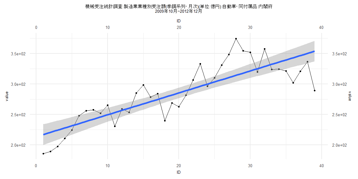
Call:
lm(formula = value ~ ID)

Residuals:
   Min     1Q Median     3Q    Max
-64.81 -17.78  -3.38  16.53  60.18

Coefficients:
            Estimate Std. Error t value             Pr(>|t|)
(Intercept) 213.3113     8.6640  24.620 < 0.0000000000000002 ***
ID            3.6020     0.3775   9.541      0.0000000000162 ***
---
Signif. codes:  0 '***' 0.001 '**' 0.01 '*' 0.05 '.' 0.1 ' ' 1

Residual standard error: 26.53 on 37 degrees of freedom
Multiple R-squared:  0.711, Adjusted R-squared:  0.7032
F-statistic: 91.03 on 1 and 37 DF,  p-value: 0.00000000001625


    Two-sample Kolmogorov-Smirnov test

data:  lm_residuals and rnorm(n = length(lm_residuals), mean = 0, sd = sd(lm_residuals))
D = 0.10256, p-value = 0.9885
alternative hypothesis: two-sided


    Durbin-Watson test

data:  value ~ ID
DW = 0.74628, p-value = 0.000001704
alternative hypothesis: true autocorrelation is greater than 0


    studentized Breusch-Pagan test

data:  value ~ ID
BP = 4.0234, df = 1, p-value = 0.04487


    Box-Ljung test

data:  lm_residuals
X-squared = 11.705, df = 1, p-value = 0.0006234
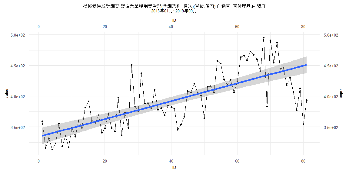
Call:
lm(formula = value ~ ID)

Residuals:
    Min      1Q  Median      3Q     Max
-95.392 -17.666   1.183  12.612  76.357

Coefficients:
            Estimate Std. Error t value             Pr(>|t|)
(Intercept)  334.248      6.937   48.18 < 0.0000000000000002 ***
ID             1.448      0.147    9.85  0.00000000000000216 ***
---
Signif. codes:  0 '***' 0.001 '**' 0.01 '*' 0.05 '.' 0.1 ' ' 1

Residual standard error: 30.93 on 79 degrees of freedom
Multiple R-squared:  0.5512,    Adjusted R-squared:  0.5455
F-statistic: 97.02 on 1 and 79 DF,  p-value: 0.000000000000002156


    Two-sample Kolmogorov-Smirnov test

data:  lm_residuals and rnorm(n = length(lm_residuals), mean = 0, sd = sd(lm_residuals))
D = 0.1358, p-value = 0.4462
alternative hypothesis: two-sided


    Durbin-Watson test

data:  value ~ ID
DW = 1.3069, p-value = 0.0004066
alternative hypothesis: true autocorrelation is greater than 0


    studentized Breusch-Pagan test

data:  value ~ ID
BP = 11.208, df = 1, p-value = 0.0008145


    Box-Ljung test

data:  lm_residuals
X-squared = 8.6444, df = 1, p-value = 0.003281
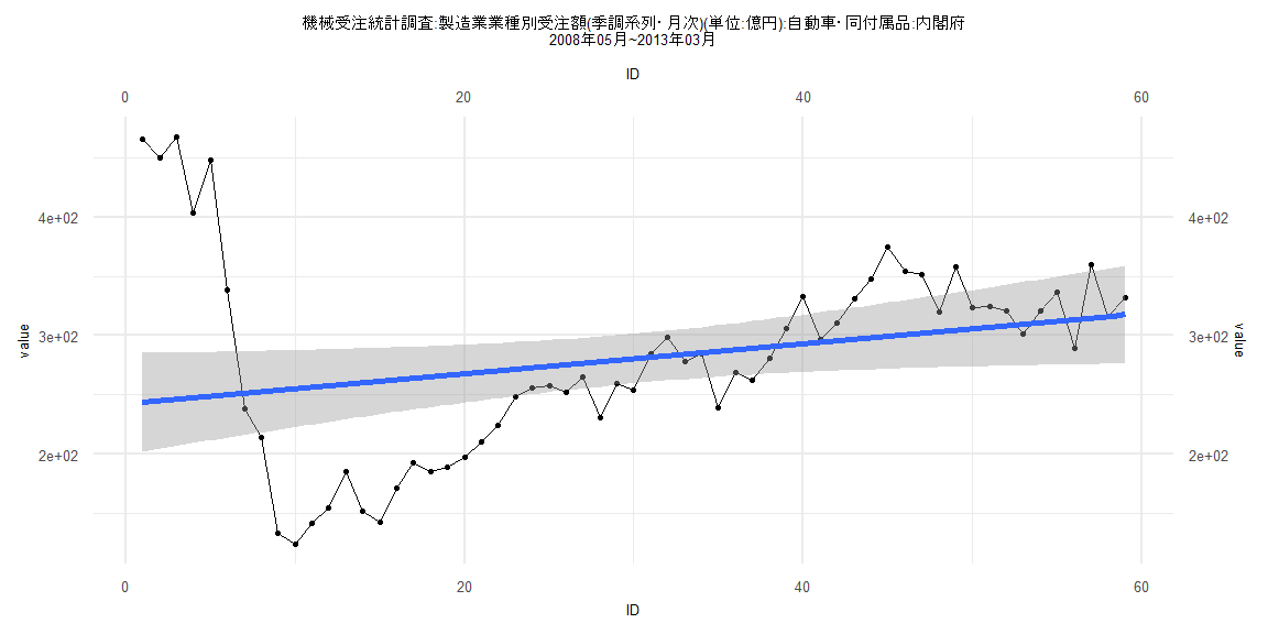
Call:
lm(formula = value ~ ID)

Residuals:
     Min       1Q   Median       3Q      Max
-131.251  -46.796   -8.281   20.766  221.910

Coefficients:
            Estimate Std. Error t value             Pr(>|t|)
(Intercept) 242.4250    21.2335  11.417 0.000000000000000234 ***
ID            1.2746     0.6155   2.071               0.0429 *
---
Signif. codes:  0 '***' 0.001 '**' 0.01 '*' 0.05 '.' 0.1 ' ' 1

Residual standard error: 80.51 on 57 degrees of freedom
Multiple R-squared:  0.06997,   Adjusted R-squared:  0.05365
F-statistic: 4.288 on 1 and 57 DF,  p-value: 0.04292


    Two-sample Kolmogorov-Smirnov test

data:  lm_residuals and rnorm(n = length(lm_residuals), mean = 0, sd = sd(lm_residuals))
D = 0.18644, p-value = 0.2582
alternative hypothesis: two-sided


    Durbin-Watson test

data:  value ~ ID
DW = 0.18195, p-value < 0.00000000000000022
alternative hypothesis: true autocorrelation is greater than 0


    studentized Breusch-Pagan test

data:  value ~ ID
BP = 23.521, df = 1, p-value = 0.000001235


    Box-Ljung test

data:  lm_residuals
X-squared = 44.004, df = 1, p-value = 0.00000000003278
Call:
lm(formula = value ~ ID)

Residuals:
    Min      1Q  Median      3Q     Max
-95.337 -17.782   1.459  12.544  76.278

Coefficients:
            Estimate Std. Error t value             Pr(>|t|)
(Intercept) 338.7348     7.1598  47.310 < 0.0000000000000002 ***
ID            1.4451     0.1575   9.177   0.0000000000000613 ***
---
Signif. codes:  0 '***' 0.001 '**' 0.01 '*' 0.05 '.' 0.1 ' ' 1

Residual standard error: 31.31 on 76 degrees of freedom
Multiple R-squared:  0.5256,    Adjusted R-squared:  0.5194
F-statistic: 84.21 on 1 and 76 DF,  p-value: 0.00000000000006133


    Two-sample Kolmogorov-Smirnov test

data:  lm_residuals and rnorm(n = length(lm_residuals), mean = 0, sd = sd(lm_residuals))
D = 0.12821, p-value = 0.546
alternative hypothesis: two-sided


    Durbin-Watson test

data:  value ~ ID
DW = 1.2905, p-value = 0.0003743
alternative hypothesis: true autocorrelation is greater than 0


    studentized Breusch-Pagan test

data:  value ~ ID
BP = 10.572, df = 1, p-value = 0.001148


    Box-Ljung test

data:  lm_residuals
X-squared = 8.7066, df = 1, p-value = 0.003171