Analysis
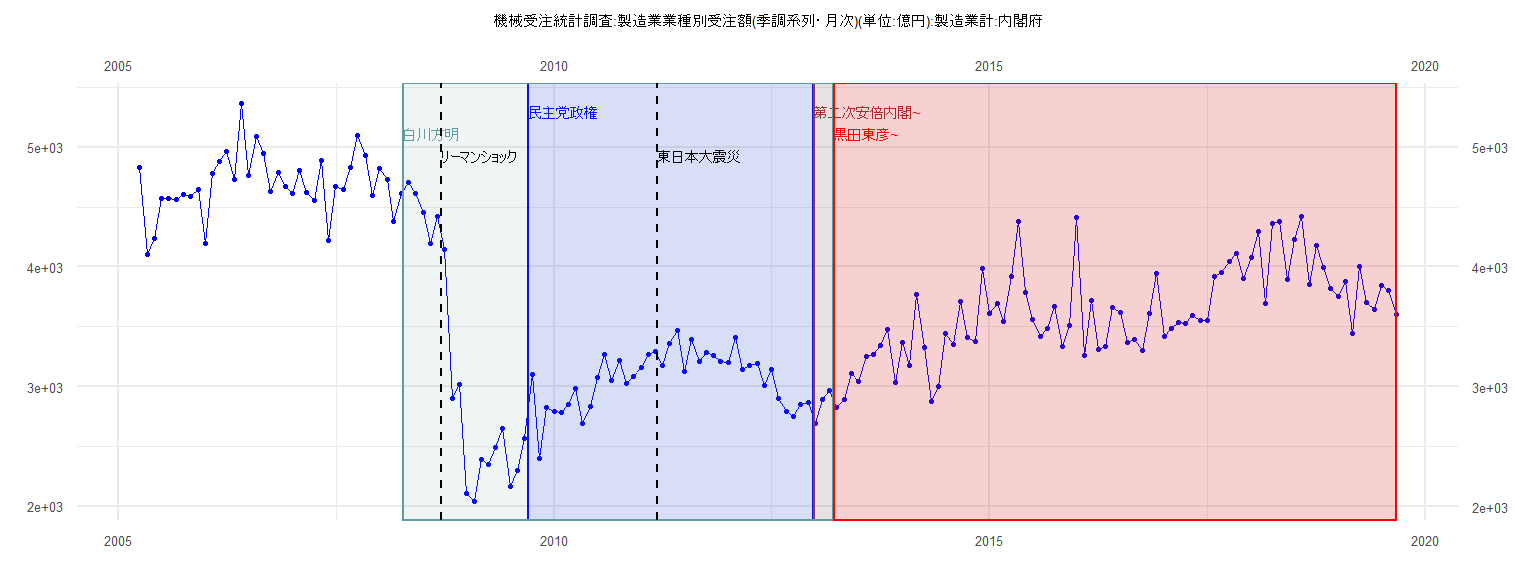
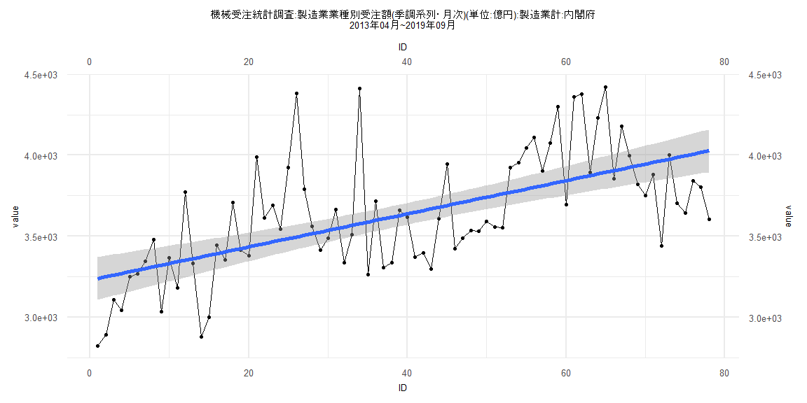
[1] "機械受注統計調査:製造業業種別受注額(季調系列・月次)(単位:億円):製造業計:内閣府"
         Jan     Feb     Mar     Apr     May     Jun     Jul     Aug     Sep     Oct     Nov     Dec
2005                         4827.59 4105.29 4239.97 4572.19 4568.84 4563.79 4606.54 4591.43 4646.57
2006 4198.65 4780.75 4881.66 4965.91 4733.10 5364.14 4762.07 5087.51 4944.06 4627.67 4791.50 4673.72
2007 4616.36 4803.53 4623.63 4553.97 4884.60 4219.32 4673.76 4650.19 4832.95 5100.21 4934.39 4592.47
2008 4817.52 4730.37 4377.54 4616.27 4708.66 4609.55 4455.45 4193.51 4417.91 4144.04 2904.49 3014.63
2009 2109.63 2044.04 2387.98 2353.37 2490.26 2650.51 2168.70 2302.45 2568.79 3104.50 2403.28 2823.39
2010 2792.97 2785.22 2849.56 2980.18 2693.84 2834.92 3075.93 3272.20 3050.08 3214.53 3022.25 3085.63
2011 3157.92 3272.26 3290.97 3177.46 3360.80 3468.92 3125.72 3395.22 3207.43 3284.97 3257.13 3212.57
2012 3202.52 3410.16 3138.68 3175.36 3196.85 3005.95 3146.95 2897.91 2794.56 2751.01 2853.34 2864.80
2013 2694.62 2890.38 2964.18 2822.48 2891.48 3107.48 3043.65 3252.08 3268.97 3344.34 3477.77 3034.37
2014 3367.94 3180.30 3772.38 3330.39 2877.68 3001.27 3442.61 3355.39 3707.40 3412.70 3379.67 3989.73
2015 3612.35 3689.95 3543.67 3922.51 4381.48 3789.75 3559.53 3415.32 3488.93 3665.28 3337.79 3507.22
2016 4413.00 3261.08 3715.76 3306.99 3335.68 3660.62 3615.94 3369.74 3396.42 3297.90 3609.49 3947.24
2017 3421.81 3485.81 3534.42 3530.80 3591.64 3554.85 3553.00 3922.26 3953.95 4043.29 4111.17 3904.69
2018 4074.66 4299.41 3695.50 4361.04 4379.89 3893.85 4231.11 4420.94 3854.53 4181.08 3996.80 3821.43
2019 3749.60 3880.73 3439.91 4000.99 3705.95 3643.90 3841.10 3801.85 3603.81
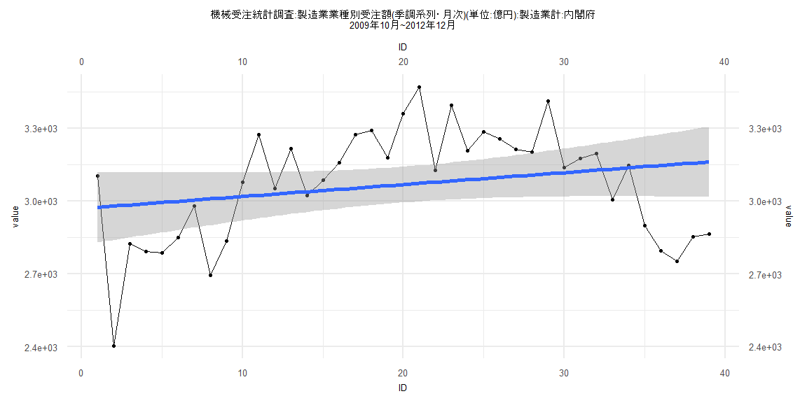
Call:
lm(formula = value ~ ID)

Residuals:
    Min      1Q  Median      3Q     Max
-575.74 -169.56   48.23  145.18  396.36

Coefficients:
            Estimate Std. Error t value            Pr(>|t|)
(Intercept) 2969.177     74.304  39.960 <0.0000000000000002 ***
ID             4.923      3.238   1.521               0.137
---
Signif. codes:  0 '***' 0.001 '**' 0.01 '*' 0.05 '.' 0.1 ' ' 1

Residual standard error: 227.6 on 37 degrees of freedom
Multiple R-squared:  0.05881,   Adjusted R-squared:  0.03338
F-statistic: 2.312 on 1 and 37 DF,  p-value: 0.1369


    Two-sample Kolmogorov-Smirnov test

data:  lm_residuals and rnorm(n = length(lm_residuals), mean = 0, sd = sd(lm_residuals))
D = 0.17949, p-value = 0.5622
alternative hypothesis: two-sided


    Durbin-Watson test

data:  value ~ ID
DW = 0.82516, p-value = 0.000009001
alternative hypothesis: true autocorrelation is greater than 0


    studentized Breusch-Pagan test

data:  value ~ ID
BP = 0.000036185, df = 1, p-value = 0.9952


    Box-Ljung test

data:  lm_residuals
X-squared = 13.199, df = 1, p-value = 0.0002801
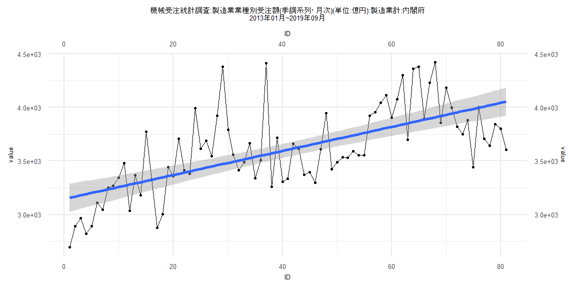
Call:
lm(formula = value ~ ID)

Residuals:
    Min      1Q  Median      3Q     Max
-545.77 -213.64  -22.54  170.24  911.95

Coefficients:
            Estimate Std. Error t value             Pr(>|t|)
(Intercept) 3144.133     66.996  46.930 < 0.0000000000000002 ***
ID            11.221      1.419   7.905      0.0000000000134 ***
---
Signif. codes:  0 '***' 0.001 '**' 0.01 '*' 0.05 '.' 0.1 ' ' 1

Residual standard error: 298.7 on 79 degrees of freedom
Multiple R-squared:  0.4416,    Adjusted R-squared:  0.4346
F-statistic: 62.49 on 1 and 79 DF,  p-value: 0.00000000001335


    Two-sample Kolmogorov-Smirnov test

data:  lm_residuals and rnorm(n = length(lm_residuals), mean = 0, sd = sd(lm_residuals))
D = 0.08642, p-value = 0.9254
alternative hypothesis: two-sided


    Durbin-Watson test

data:  value ~ ID
DW = 1.2843, p-value = 0.0002687
alternative hypothesis: true autocorrelation is greater than 0


    studentized Breusch-Pagan test

data:  value ~ ID
BP = 0.016672, df = 1, p-value = 0.8973


    Box-Ljung test

data:  lm_residuals
X-squared = 9.0678, df = 1, p-value = 0.002602
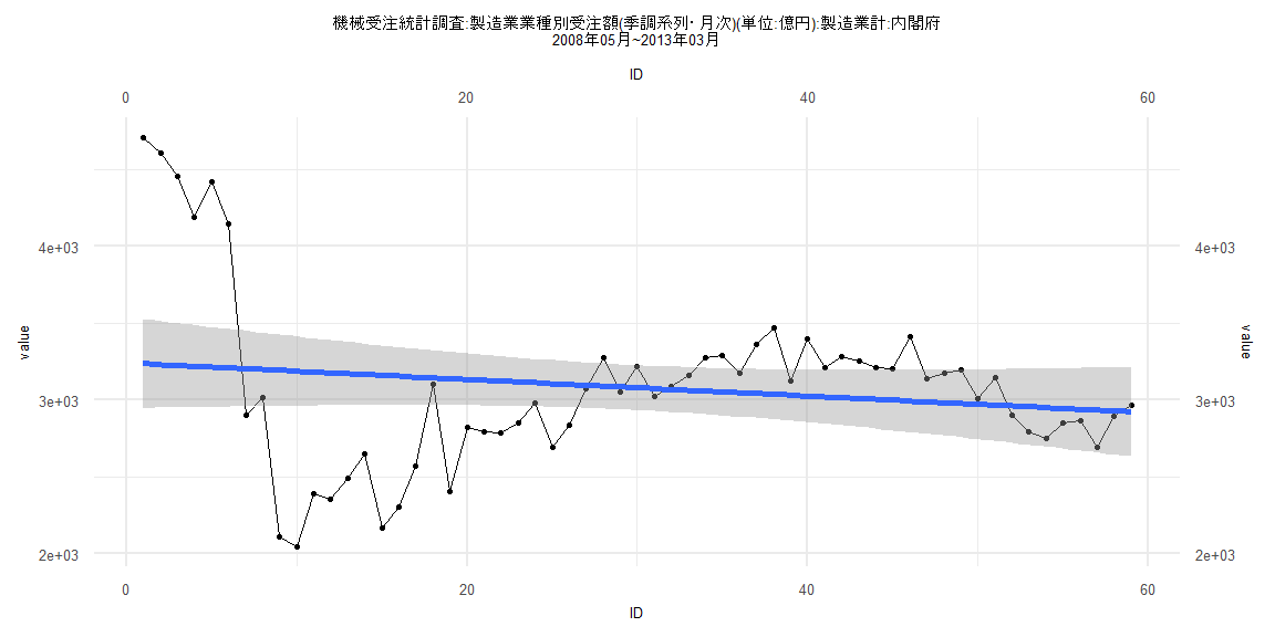
Call:
lm(formula = value ~ ID)

Residuals:
     Min       1Q   Median       3Q      Max
-1143.77  -283.80   -20.11   211.15  1472.27

Coefficients:
            Estimate Std. Error t value            Pr(>|t|)
(Intercept) 3241.792    148.498  21.831 <0.0000000000000002 ***
ID            -5.398      4.305  -1.254               0.215
---
Signif. codes:  0 '***' 0.001 '**' 0.01 '*' 0.05 '.' 0.1 ' ' 1

Residual standard error: 563.1 on 57 degrees of freedom
Multiple R-squared:  0.02685,   Adjusted R-squared:  0.009774
F-statistic: 1.572 on 1 and 57 DF,  p-value: 0.215


    Two-sample Kolmogorov-Smirnov test

data:  lm_residuals and rnorm(n = length(lm_residuals), mean = 0, sd = sd(lm_residuals))
D = 0.15254, p-value = 0.5021
alternative hypothesis: two-sided


    Durbin-Watson test

data:  value ~ ID
DW = 0.27692, p-value < 0.00000000000000022
alternative hypothesis: true autocorrelation is greater than 0


    studentized Breusch-Pagan test

data:  value ~ ID
BP = 28.181, df = 1, p-value = 0.0000001105


    Box-Ljung test

data:  lm_residuals
X-squared = 39.864, df = 1, p-value = 0.0000000002722
Call:
lm(formula = value ~ ID)

Residuals:
   Min     1Q Median     3Q    Max
-526.1 -213.6  -39.2  165.0  886.5

Coefficients:
            Estimate Std. Error t value             Pr(>|t|)
(Intercept) 3228.687     67.709  47.685 < 0.0000000000000002 ***
ID            10.241      1.489   6.877         0.0000000015 ***
---
Signif. codes:  0 '***' 0.001 '**' 0.01 '*' 0.05 '.' 0.1 ' ' 1

Residual standard error: 296.1 on 76 degrees of freedom
Multiple R-squared:  0.3836,    Adjusted R-squared:  0.3754
F-statistic: 47.29 on 1 and 76 DF,  p-value: 0.000000001498


    Two-sample Kolmogorov-Smirnov test

data:  lm_residuals and rnorm(n = length(lm_residuals), mean = 0, sd = sd(lm_residuals))
D = 0.11538, p-value = 0.6802
alternative hypothesis: two-sided


    Durbin-Watson test

data:  value ~ ID
DW = 1.349, p-value = 0.001013
alternative hypothesis: true autocorrelation is greater than 0


    studentized Breusch-Pagan test

data:  value ~ ID
BP = 0.010758, df = 1, p-value = 0.9174


    Box-Ljung test

data:  lm_residuals
X-squared = 7.2457, df = 1, p-value = 0.007107