Analysis
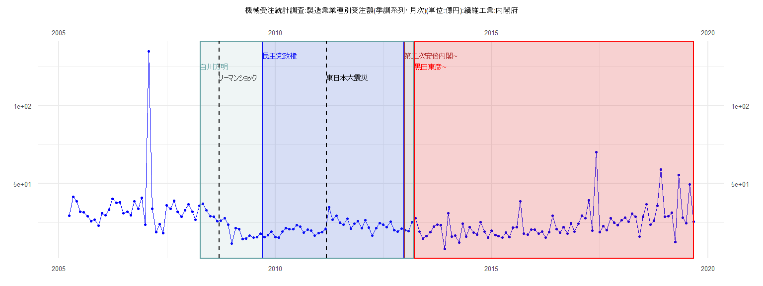
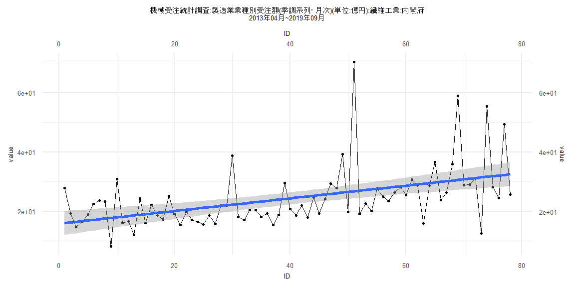
[1] "機械受注統計調査:製造業業種別受注額(季調系列・月次)(単位:億円):繊維工業:内閣府"
        Jan    Feb    Mar    Apr    May    Jun    Jul    Aug    Sep    Oct    Nov    Dec
2005                       29.52  41.43  38.67  31.90  31.69  29.08  26.03  26.91  23.15
2006  31.17  29.89  33.25  40.24  37.63  38.17  30.92  31.95  29.90  38.83  34.06  40.95
2007  23.55 134.91  33.92  18.84  24.18  18.26  36.12  33.98  39.11  31.87  28.65  32.86
2008  36.93  31.84  26.79  35.87  37.23  32.84  29.25  28.87  26.05  26.21  27.69  23.58
2009  11.75  21.34  20.89  14.39  14.86  16.60  15.51  15.64  17.92  15.80  17.15  19.32
2010  15.77  15.37  19.31  21.40  20.78  20.78  23.52  22.38  18.72  20.36  19.81  16.69
2011  18.24  18.88  20.72  34.87  26.86  29.50  25.08  23.60  27.37  21.24  24.39  25.99
2012  21.41  26.57  21.74  16.84  21.41  24.69  23.82  22.14  25.50  20.11  19.32  21.24
2013  20.04  19.66  25.16  27.87  19.23  14.84  16.46  19.02  22.50  23.68  23.32   8.23
2014  30.93  16.09  16.62  12.15  24.34  16.08  22.22  18.57  17.27  25.19  19.12  15.48
2015  19.88  17.09  16.45  15.54  18.62  15.86  21.94  22.05  38.76  18.08  17.18  20.45
2016  20.43  18.09  19.37  15.50  18.77  29.57  20.85  18.64  22.07  17.95  24.76  19.26
2017  24.25  29.31  27.87  39.26  19.78  70.38  19.08  22.74  20.12  27.77  24.94  23.53
2018  26.44  28.17  25.57  30.69  28.92  15.94  28.66  36.62  23.85  26.33  35.89  58.99
2019  28.82  29.04  31.21  12.66  55.48  28.18  24.53  49.41  25.67
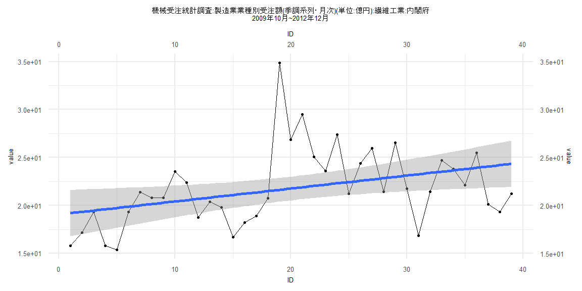
Call:
lm(formula = value ~ ID)

Residuals:
    Min      1Q  Median      3Q     Max
-6.4094 -2.3258 -0.5573  1.6956 13.2440

Coefficients:
            Estimate Std. Error t value            Pr(>|t|)
(Intercept) 19.05557    1.24192   15.34 <0.0000000000000002 ***
ID           0.13529    0.05412    2.50               0.017 *
---
Signif. codes:  0 '***' 0.001 '**' 0.01 '*' 0.05 '.' 0.1 ' ' 1

Residual standard error: 3.804 on 37 degrees of freedom
Multiple R-squared:  0.1445,    Adjusted R-squared:  0.1214
F-statistic:  6.25 on 1 and 37 DF,  p-value: 0.01698


    Two-sample Kolmogorov-Smirnov test

data:  lm_residuals and rnorm(n = length(lm_residuals), mean = 0, sd = sd(lm_residuals))
D = 0.23077, p-value = 0.2523
alternative hypothesis: two-sided


    Durbin-Watson test

data:  value ~ ID
DW = 1.1435, p-value = 0.00128
alternative hypothesis: true autocorrelation is greater than 0


    studentized Breusch-Pagan test

data:  value ~ ID
BP = 0.075198, df = 1, p-value = 0.7839


    Box-Ljung test

data:  lm_residuals
X-squared = 7.0248, df = 1, p-value = 0.008039
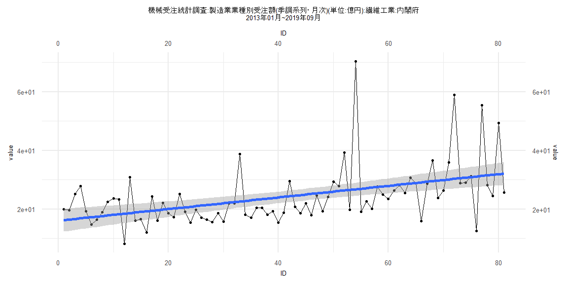
Call:
lm(formula = value ~ ID)

Residuals:
    Min      1Q  Median      3Q     Max
-18.484  -4.992  -1.734   2.362  43.592

Coefficients:
            Estimate Std. Error t value         Pr(>|t|)
(Intercept) 16.09540    2.00372   8.033 0.00000000000753 ***
ID           0.19801    0.04245   4.664 0.00001241889138 ***
---
Signif. codes:  0 '***' 0.001 '**' 0.01 '*' 0.05 '.' 0.1 ' ' 1

Residual standard error: 8.933 on 79 degrees of freedom
Multiple R-squared:  0.2159,    Adjusted R-squared:  0.206
F-statistic: 21.76 on 1 and 79 DF,  p-value: 0.00001242


    Two-sample Kolmogorov-Smirnov test

data:  lm_residuals and rnorm(n = length(lm_residuals), mean = 0, sd = sd(lm_residuals))
D = 0.22222, p-value = 0.03633
alternative hypothesis: two-sided


    Durbin-Watson test

data:  value ~ ID
DW = 2.3427, p-value = 0.9256
alternative hypothesis: true autocorrelation is greater than 0


    studentized Breusch-Pagan test

data:  value ~ ID
BP = 3.0305, df = 1, p-value = 0.08172


    Box-Ljung test

data:  lm_residuals
X-squared = 2.5963, df = 1, p-value = 0.1071
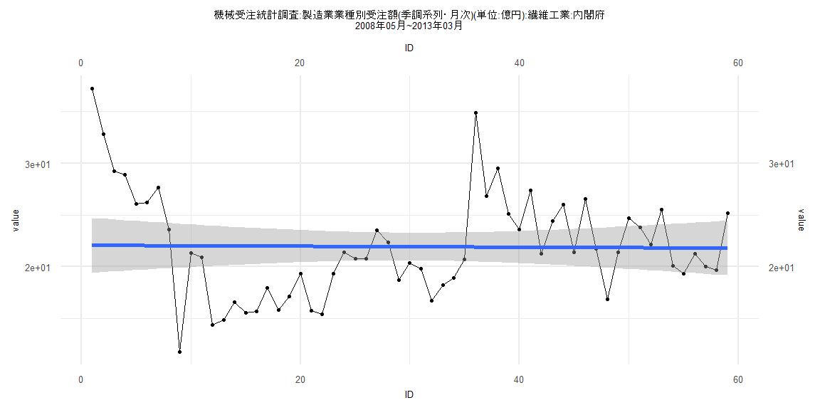
Call:
lm(formula = value ~ ID)

Residuals:
     Min       1Q   Median       3Q      Max
-10.2801  -3.1283  -0.6408   3.2709  15.1637

Coefficients:
             Estimate Std. Error t value            Pr(>|t|)
(Intercept) 22.070812   1.356851  16.266 <0.0000000000000002 ***
ID          -0.004524   0.039333  -0.115               0.909
---
Signif. codes:  0 '***' 0.001 '**' 0.01 '*' 0.05 '.' 0.1 ' ' 1

Residual standard error: 5.145 on 57 degrees of freedom
Multiple R-squared:  0.0002321, Adjusted R-squared:  -0.01731
F-statistic: 0.01323 on 1 and 57 DF,  p-value: 0.9088


    Two-sample Kolmogorov-Smirnov test

data:  lm_residuals and rnorm(n = length(lm_residuals), mean = 0, sd = sd(lm_residuals))
D = 0.16949, p-value = 0.3674
alternative hypothesis: two-sided


    Durbin-Watson test

data:  value ~ ID
DW = 0.65777, p-value = 0.0000000004473
alternative hypothesis: true autocorrelation is greater than 0


    studentized Breusch-Pagan test

data:  value ~ ID
BP = 10.247, df = 1, p-value = 0.001369


    Box-Ljung test

data:  lm_residuals
X-squared = 21.687, df = 1, p-value = 0.00000321
Call:
lm(formula = value ~ ID)

Residuals:
    Min      1Q  Median      3Q     Max
-18.811  -4.799  -2.007   2.004  43.609

Coefficients:
            Estimate Std. Error t value        Pr(>|t|)
(Intercept) 15.87440    2.06454   7.689 0.0000000000433 ***
ID           0.21365    0.04541   4.705 0.0000111446133 ***
---
Signif. codes:  0 '***' 0.001 '**' 0.01 '*' 0.05 '.' 0.1 ' ' 1

Residual standard error: 9.029 on 76 degrees of freedom
Multiple R-squared:  0.2256,    Adjusted R-squared:  0.2154
F-statistic: 22.14 on 1 and 76 DF,  p-value: 0.00001114


    Two-sample Kolmogorov-Smirnov test

data:  lm_residuals and rnorm(n = length(lm_residuals), mean = 0, sd = sd(lm_residuals))
D = 0.20513, p-value = 0.07495
alternative hypothesis: two-sided


    Durbin-Watson test

data:  value ~ ID
DW = 2.3782, p-value = 0.9423
alternative hypothesis: true autocorrelation is greater than 0


    studentized Breusch-Pagan test

data:  value ~ ID
BP = 2.7805, df = 1, p-value = 0.09542


    Box-Ljung test

data:  lm_residuals
X-squared = 3.3761, df = 1, p-value = 0.06615