Analysis
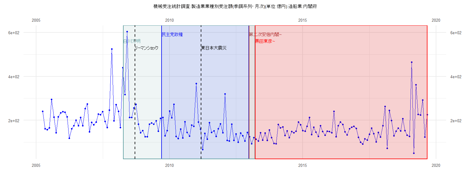
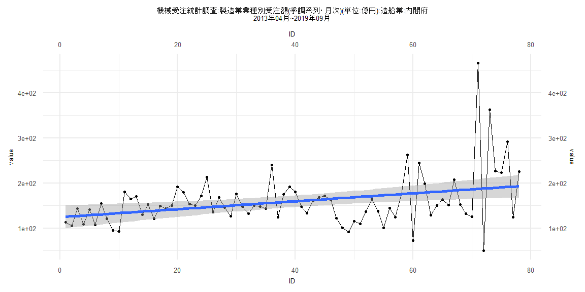
[1] "機械受注統計調査:製造業業種別受注額(季調系列・月次)(単位:億円):造船業:内閣府"
        Jan    Feb    Mar    Apr    May    Jun    Jul    Aug    Sep    Oct    Nov    Dec
2005                      241.10 161.42 157.45 165.95 294.37 214.33 143.24 215.38 233.33
2006 238.99 236.14 215.24 118.15 160.85 175.26 200.31 175.33 212.82 174.61 252.59 274.22
2007 146.96 190.49 179.04 192.43 227.45 225.60 239.08 194.31 167.11 246.46 524.89 198.06
2008 270.66 240.86 167.30 439.48 317.11 603.92 212.58 212.16 255.95 273.26 182.36 142.57
2009 152.80 124.69 125.28 181.45 187.64 182.15 198.02 150.79 208.44 212.53 129.57 153.27
2010 241.78 211.90 272.53 126.96 116.05 160.51 119.53 192.70 144.64 127.35 178.40 171.83
2011 367.16 191.42 159.42  66.62 140.15 113.71 188.71 144.45 151.13 126.72 161.31 183.76
2012 143.33 319.52 107.67 104.96 182.19 108.10 137.89 100.52 141.14 129.73 105.58 145.03
2013 125.68  93.11 120.36 113.70 105.22 143.15 109.09 141.59 107.88 155.10 121.54  94.82
2014  93.29 180.15 165.13 170.10 129.95 152.07 121.33 149.24 143.22 149.76 191.72 179.83
2015 153.06 150.62 171.85 212.71 135.39 167.79 146.29 126.18 175.79 148.29 132.29 150.31
2016 148.38 143.01 240.28 124.80 175.12 192.18 180.62 147.74 133.67 160.75 168.67 172.09
2017 162.46 122.62 100.60  92.00 115.40 110.07 136.66 164.63 138.29 101.17 144.90 124.12
2018 175.29 262.26  72.43 244.24 198.78 128.56 150.66 163.33 150.97 207.18 152.83 132.24
2019 126.03 465.43  50.47 362.21 226.16 223.25 292.12 124.12 224.89
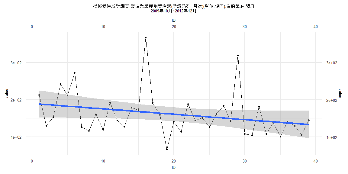
Call:
lm(formula = value ~ ID)

Residuals:
    Min      1Q  Median      3Q     Max
-95.850 -36.409  -6.089  21.295 200.340

Coefficients:
            Estimate Std. Error t value         Pr(>|t|)
(Intercept) 190.0207    18.9022  10.053 0.00000000000397 ***
ID           -1.4500     0.8237  -1.761           0.0866 .
---
Signif. codes:  0 '***' 0.001 '**' 0.01 '*' 0.05 '.' 0.1 ' ' 1

Residual standard error: 57.89 on 37 degrees of freedom
Multiple R-squared:  0.07729,   Adjusted R-squared:  0.05235
F-statistic: 3.099 on 1 and 37 DF,  p-value: 0.08659


    Two-sample Kolmogorov-Smirnov test

data:  lm_residuals and rnorm(n = length(lm_residuals), mean = 0, sd = sd(lm_residuals))
D = 0.17949, p-value = 0.5622
alternative hypothesis: two-sided


    Durbin-Watson test

data:  value ~ ID
DW = 1.9777, p-value = 0.4042
alternative hypothesis: true autocorrelation is greater than 0


    studentized Breusch-Pagan test

data:  value ~ ID
BP = 0.12882, df = 1, p-value = 0.7197


    Box-Ljung test

data:  lm_residuals
X-squared = 0.0028894, df = 1, p-value = 0.9571
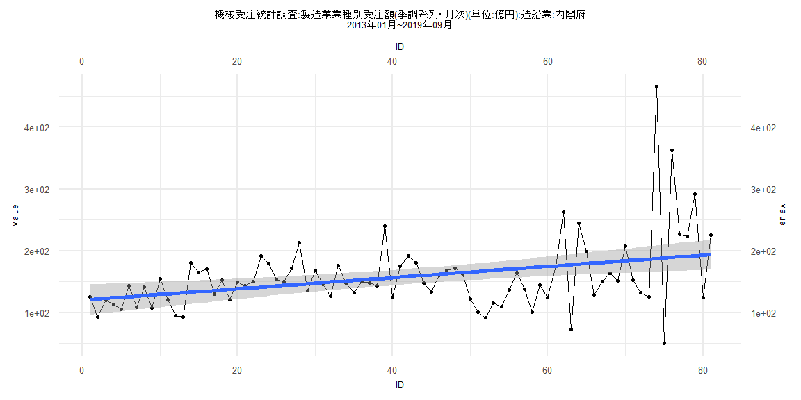
Call:
lm(formula = value ~ ID)

Residuals:
     Min       1Q   Median       3Q      Max
-137.905  -30.462   -2.731   21.260  277.961

Coefficients:
            Estimate Std. Error t value            Pr(>|t|)
(Intercept) 120.3708    12.4539   9.665 0.00000000000000492 ***
ID            0.9067     0.2639   3.436            0.000943 ***
---
Signif. codes:  0 '***' 0.001 '**' 0.01 '*' 0.05 '.' 0.1 ' ' 1

Residual standard error: 55.52 on 79 degrees of freedom
Multiple R-squared:   0.13, Adjusted R-squared:  0.119
F-statistic: 11.81 on 1 and 79 DF,  p-value: 0.0009429


    Two-sample Kolmogorov-Smirnov test

data:  lm_residuals and rnorm(n = length(lm_residuals), mean = 0, sd = sd(lm_residuals))
D = 0.23457, p-value = 0.02289
alternative hypothesis: two-sided


    Durbin-Watson test

data:  value ~ ID
DW = 2.5116, p-value = 0.9873
alternative hypothesis: true autocorrelation is greater than 0


    studentized Breusch-Pagan test

data:  value ~ ID
BP = 8.4497, df = 1, p-value = 0.003651


    Box-Ljung test

data:  lm_residuals
X-squared = 5.5864, df = 1, p-value = 0.0181
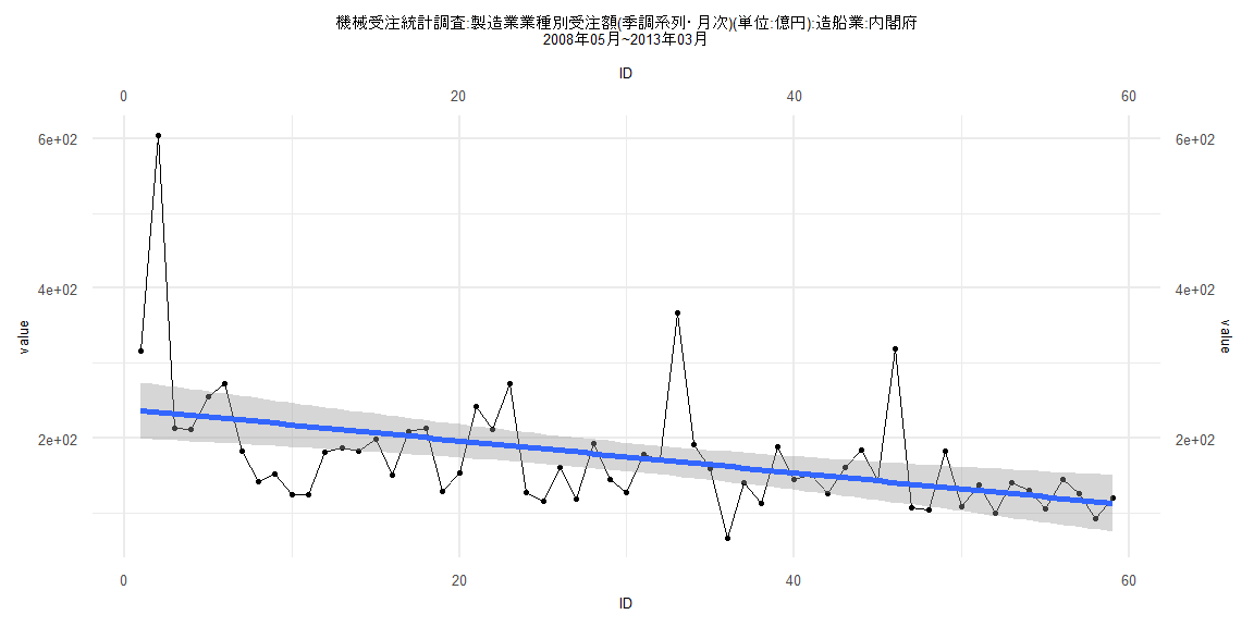
Call:
lm(formula = value ~ ID)

Residuals:
   Min     1Q Median     3Q    Max
-95.63 -32.37  -9.24  14.65 368.93

Coefficients:
            Estimate Std. Error t value             Pr(>|t|)
(Intercept)  239.273     19.388  12.341 < 0.0000000000000002 ***
ID            -2.140      0.562  -3.807             0.000346 ***
---
Signif. codes:  0 '***' 0.001 '**' 0.01 '*' 0.05 '.' 0.1 ' ' 1

Residual standard error: 73.52 on 57 degrees of freedom
Multiple R-squared:  0.2027,    Adjusted R-squared:  0.1887
F-statistic: 14.49 on 1 and 57 DF,  p-value: 0.0003463


    Two-sample Kolmogorov-Smirnov test

data:  lm_residuals and rnorm(n = length(lm_residuals), mean = 0, sd = sd(lm_residuals))
D = 0.23729, p-value = 0.07193
alternative hypothesis: two-sided


    Durbin-Watson test

data:  value ~ ID
DW = 1.6372, p-value = 0.06056
alternative hypothesis: true autocorrelation is greater than 0


    studentized Breusch-Pagan test

data:  value ~ ID
BP = 2.8731, df = 1, p-value = 0.09007


    Box-Ljung test

data:  lm_residuals
X-squared = 1.813, df = 1, p-value = 0.1782
Call:
lm(formula = value ~ ID)

Residuals:
     Min       1Q   Median       3Q      Max
-137.350  -31.139   -3.367   23.046  278.488

Coefficients:
            Estimate Std. Error t value            Pr(>|t|)
(Intercept) 124.5439    12.9196   9.640 0.00000000000000801 ***
ID            0.8788     0.2842   3.093             0.00277 **
---
Signif. codes:  0 '***' 0.001 '**' 0.01 '*' 0.05 '.' 0.1 ' ' 1

Residual standard error: 56.5 on 76 degrees of freedom
Multiple R-squared:  0.1118,    Adjusted R-squared:  0.1001
F-statistic: 9.565 on 1 and 76 DF,  p-value: 0.002773


    Two-sample Kolmogorov-Smirnov test

data:  lm_residuals and rnorm(n = length(lm_residuals), mean = 0, sd = sd(lm_residuals))
D = 0.14103, p-value = 0.4221
alternative hypothesis: two-sided


    Durbin-Watson test

data:  value ~ ID
DW = 2.5134, p-value = 0.986
alternative hypothesis: true autocorrelation is greater than 0


    studentized Breusch-Pagan test

data:  value ~ ID
BP = 8.1086, df = 1, p-value = 0.004406


    Box-Ljung test

data:  lm_residuals
X-squared = 5.4379, df = 1, p-value = 0.0197