Analysis
[1] "機械受注統計調査:製造業業種別受注額(季調系列・月次)(単位:億円):鉄鋼業:内閣府"
         Jan     Feb     Mar     Apr     May     Jun     Jul     Aug     Sep     Oct     Nov     Dec
2005                          168.39  186.16  107.98  151.66  121.95  147.02  104.11  173.92  147.63
2006  135.15  167.20  100.41  150.37   98.45  422.49  130.01  139.93  142.96  144.30  152.04  119.14
2007  116.86  113.32  200.03  202.60  210.06  203.57  195.32  154.93  211.94  213.12  212.85  158.97
2008  539.63  192.00  164.32  171.57  376.67  185.25  235.84  194.63  122.16  206.74  118.85  513.31
2009  136.91  163.31   74.26  105.03   76.19  114.82   79.50   97.89  104.22   91.69   72.69  149.87
2010  181.04   85.78  122.02   81.49  101.34  132.91   98.36  189.00  107.17   89.35  103.18   87.03
2011   83.55   92.60  157.49  105.40  108.50  112.89   81.86  104.95  130.70  123.02  136.69  139.65
2012   92.19   93.42  129.55   89.88   85.35   91.84  191.47   75.23   98.04   74.58  109.21   78.36
2013   71.10   93.75   84.75   94.08   80.74   72.46   97.47   99.85   99.96   86.85   95.16   80.12
2014   83.10   97.72   89.11  106.16   83.18   84.13   94.66  104.47   94.38  111.66   82.77   82.24
2015   88.00  101.05   97.97  100.81 1003.84  111.76  176.67   90.90   93.97  173.03  104.22  126.53
2016 1458.52   90.20  122.95  120.98  108.24  133.08  235.84   83.90  108.64  120.52  137.46  115.38
2017  114.74  107.19  115.83  112.38  110.15  131.33  104.90  128.29  121.83  114.90  117.39  129.70
2018   94.31  171.14  116.63  148.12  144.65  111.32  103.89  165.68  138.03   87.54  125.51  145.03
2019  109.87   97.64  134.43  139.14  120.62  118.07  144.84  123.48  131.68
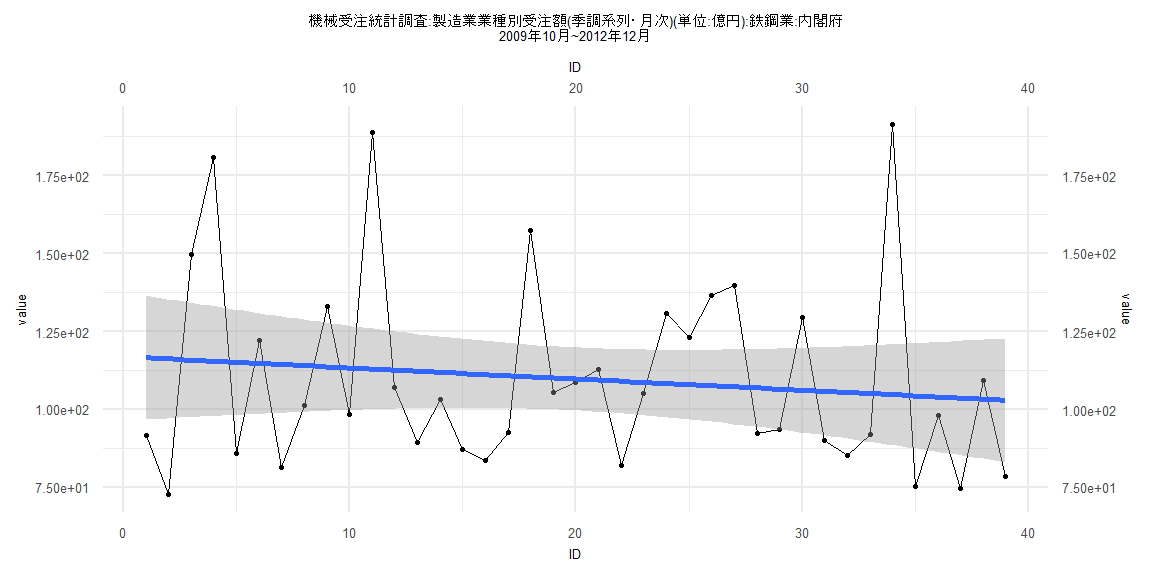
Call:
lm(formula = value ~ ID)

Residuals:
    Min      1Q  Median      3Q     Max
-43.499 -23.691  -8.701  17.161  86.770

Coefficients:
            Estimate Std. Error t value           Pr(>|t|)
(Intercept) 116.9073    10.2006  11.461 0.0000000000000983 ***
ID           -0.3590     0.4445  -0.808              0.424
---
Signif. codes:  0 '***' 0.001 '**' 0.01 '*' 0.05 '.' 0.1 ' ' 1

Residual standard error: 31.24 on 37 degrees of freedom
Multiple R-squared:  0.01733,   Adjusted R-squared:  -0.00923
F-statistic: 0.6525 on 1 and 37 DF,  p-value: 0.4244


    Two-sample Kolmogorov-Smirnov test

data:  lm_residuals and rnorm(n = length(lm_residuals), mean = 0, sd = sd(lm_residuals))
D = 0.12821, p-value = 0.9114
alternative hypothesis: two-sided


    Durbin-Watson test

data:  value ~ ID
DW = 2.1848, p-value = 0.6596
alternative hypothesis: true autocorrelation is greater than 0


    studentized Breusch-Pagan test

data:  value ~ ID
BP = 0.27575, df = 1, p-value = 0.5995


    Box-Ljung test

data:  lm_residuals
X-squared = 0.50282, df = 1, p-value = 0.4783
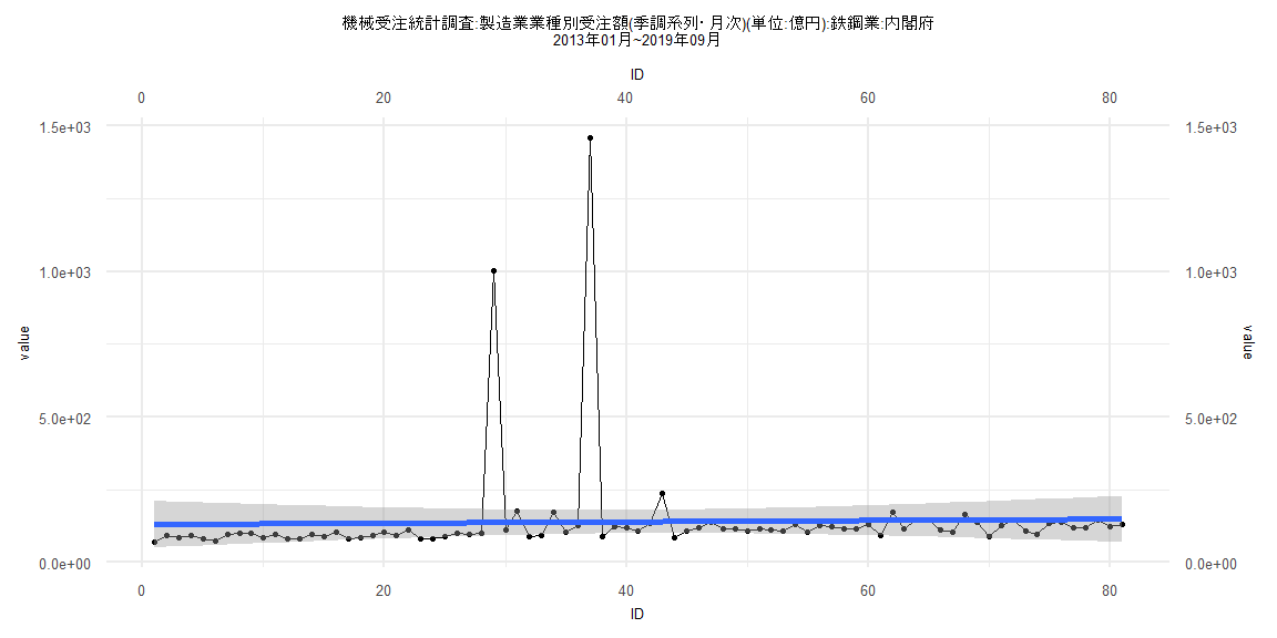
Call:
lm(formula = value ~ ID)

Residuals:
    Min      1Q  Median      3Q     Max
 -59.86  -42.28  -31.94  -16.77 1319.26

Coefficients:
            Estimate Std. Error t value Pr(>|t|)
(Intercept) 130.7304    40.6867   3.213   0.0019 **
ID            0.2305     0.8620   0.267   0.7899
---
Signif. codes:  0 '***' 0.001 '**' 0.01 '*' 0.05 '.' 0.1 ' ' 1

Residual standard error: 181.4 on 79 degrees of freedom
Multiple R-squared:  0.000904,  Adjusted R-squared:  -0.01174
F-statistic: 0.07148 on 1 and 79 DF,  p-value: 0.7899


    Two-sample Kolmogorov-Smirnov test

data:  lm_residuals and rnorm(n = length(lm_residuals), mean = 0, sd = sd(lm_residuals))
D = 0.45679, p-value = 0.00000005397
alternative hypothesis: two-sided


    Durbin-Watson test

data:  value ~ ID
DW = 2.0582, p-value = 0.5588
alternative hypothesis: true autocorrelation is greater than 0


    studentized Breusch-Pagan test

data:  value ~ ID
BP = 0.1476, df = 1, p-value = 0.7008


    Box-Ljung test

data:  lm_residuals
X-squared = 0.074931, df = 1, p-value = 0.7843
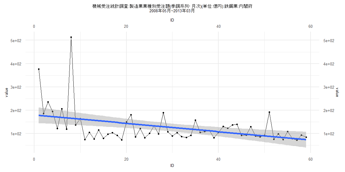
Call:
lm(formula = value ~ ID)

Residuals:
   Min     1Q Median     3Q    Max
-86.05 -36.01  -6.16  18.48 347.58

Coefficients:
            Estimate Std. Error t value           Pr(>|t|)
(Intercept) 180.1690    17.3759  10.369 0.0000000000000098 ***
ID           -1.8053     0.5037  -3.584           0.000701 ***
---
Signif. codes:  0 '***' 0.001 '**' 0.01 '*' 0.05 '.' 0.1 ' ' 1

Residual standard error: 65.89 on 57 degrees of freedom
Multiple R-squared:  0.1839,    Adjusted R-squared:  0.1696
F-statistic: 12.85 on 1 and 57 DF,  p-value: 0.0007015


    Two-sample Kolmogorov-Smirnov test

data:  lm_residuals and rnorm(n = length(lm_residuals), mean = 0, sd = sd(lm_residuals))
D = 0.27119, p-value = 0.02566
alternative hypothesis: two-sided


    Durbin-Watson test

data:  value ~ ID
DW = 1.8213, p-value = 0.2038
alternative hypothesis: true autocorrelation is greater than 0


    studentized Breusch-Pagan test

data:  value ~ ID
BP = 4.2364, df = 1, p-value = 0.03957


    Box-Ljung test

data:  lm_residuals
X-squared = 0.0057529, df = 1, p-value = 0.9395
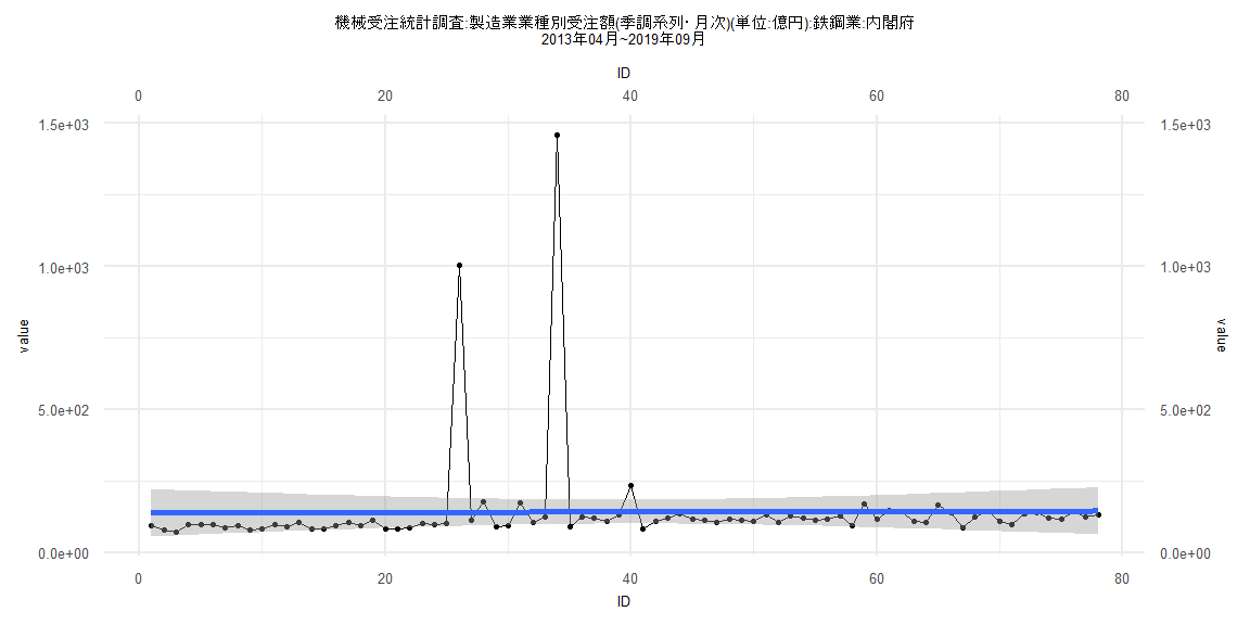
Call:
lm(formula = value ~ ID)

Residuals:
    Min      1Q  Median      3Q     Max
 -66.89  -45.60  -33.04  -15.22 1316.60

Coefficients:
             Estimate Std. Error t value Pr(>|t|)
(Intercept) 139.10592   42.21977   3.295   0.0015 **
ID            0.08267    0.92860   0.089   0.9293
---
Signif. codes:  0 '***' 0.001 '**' 0.01 '*' 0.05 '.' 0.1 ' ' 1

Residual standard error: 184.6 on 76 degrees of freedom
Multiple R-squared:  0.0001043, Adjusted R-squared:  -0.01305
F-statistic: 0.007926 on 1 and 76 DF,  p-value: 0.9293


    Two-sample Kolmogorov-Smirnov test

data:  lm_residuals and rnorm(n = length(lm_residuals), mean = 0, sd = sd(lm_residuals))
D = 0.44872, p-value = 0.0000001903
alternative hypothesis: two-sided


    Durbin-Watson test

data:  value ~ ID
DW = 2.0646, p-value = 0.567
alternative hypothesis: true autocorrelation is greater than 0


    studentized Breusch-Pagan test

data:  value ~ ID
BP = 0.24437, df = 1, p-value = 0.6211


    Box-Ljung test

data:  lm_residuals
X-squared = 0.086687, df = 1, p-value = 0.7684