Analysis
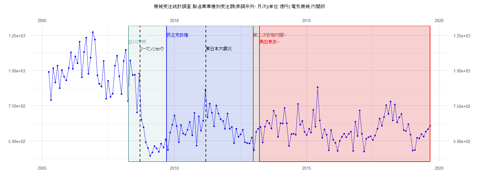
[1] "機械受注統計調査:製造業業種別受注額(季調系列・月次)(単位:億円):電気機械:内閣府"
Jan Feb Mar Apr May Jun Jul Aug Sep Oct Nov Dec
2005 991.84 792.80 1018.32 915.86 1034.36 875.67 1005.15 957.54 930.36
2006 1017.81 1130.86 1012.91 1100.99 1052.91 1205.80 952.80 1131.73 1233.68 977.68 1091.77 1273.70
2007 1221.21 966.04 906.46 886.34 1069.15 800.58 927.31 814.25 835.96 1034.35 1106.90 960.79
2008 833.67 1068.33 1148.64 783.85 1071.75 968.81 970.15 703.92 980.16 651.52 597.66 491.27
2009 449.03 395.12 418.81 463.52 447.56 423.94 481.36 453.11 511.92 435.06 560.47 614.56
2010 681.92 606.35 490.62 613.46 552.38 544.94 580.67 635.48 540.80 699.41 466.59 674.83
2011 572.70 643.73 864.49 667.27 766.29 702.07 604.80 752.90 694.52 654.77 642.46 586.04
2012 693.92 587.36 599.67 484.84 586.60 528.62 546.45 579.21 490.90 484.68 483.24 523.48
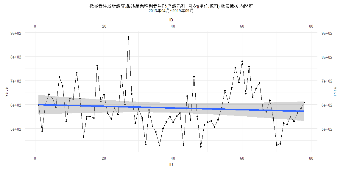
2013 433.62 565.11 587.41 599.20 490.23 602.26 644.12 626.02 588.69 715.25 679.00 530.04
2014 625.76 623.85 734.90 626.70 464.78 549.53 550.96 544.47 762.97 614.25 642.63 565.13
2015 541.51 585.53 559.30 720.43 601.45 882.89 645.32 522.21 581.45 544.55 434.63 577.61
2016 509.90 486.97 428.84 500.21 528.17 551.06 526.74 551.93 566.18 430.39 636.53 536.20
2017 716.38 550.66 424.57 516.25 527.19 532.81 507.16 536.74 587.06 660.10 609.20 670.89
2018 754.97 693.22 781.96 646.90 759.49 631.97 669.17 692.44 578.51 570.16 619.39 545.31
2019 432.47 437.23 523.38 516.87 549.17 530.51 565.60 584.26 609.18
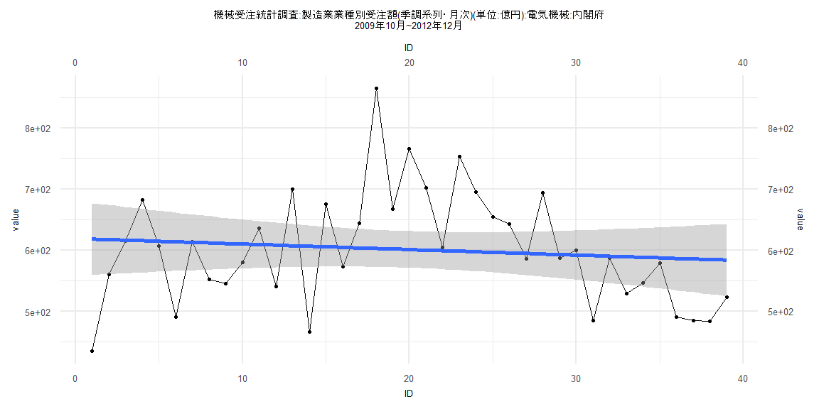
Call:
lm(formula = value ~ ID)

Residuals:
     Min       1Q   Median       3Q      Max
-183.159  -60.429   -5.467   61.845  261.688

Coefficients:
            Estimate Std. Error t value            Pr(>|t|)
(Intercept) 619.1256    30.1530   20.53 <0.0000000000000002 ***
ID           -0.9069     1.3139   -0.69               0.494
---
Signif. codes:  0 '***' 0.001 '**' 0.01 '*' 0.05 '.' 0.1 ' ' 1

Residual standard error: 92.35 on 37 degrees of freedom
Multiple R-squared:  0.01271,   Adjusted R-squared:  -0.01397
F-statistic: 0.4764 on 1 and 37 DF,  p-value: 0.4944


    Two-sample Kolmogorov-Smirnov test

data:  lm_residuals and rnorm(n = length(lm_residuals), mean = 0, sd = sd(lm_residuals))
D = 0.17949, p-value = 0.5622
alternative hypothesis: two-sided


    Durbin-Watson test

data:  value ~ ID
DW = 1.3152, p-value = 0.008149
alternative hypothesis: true autocorrelation is greater than 0


    studentized Breusch-Pagan test

data:  value ~ ID
BP = 0.2822, df = 1, p-value = 0.5953


    Box-Ljung test

data:  lm_residuals
X-squared = 3.3821, df = 1, p-value = 0.06591
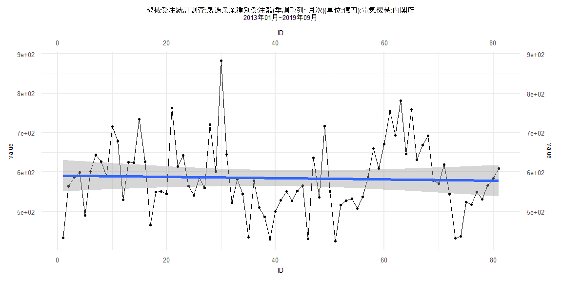
Call:
lm(formula = value ~ ID)

Residuals:
     Min       1Q   Median       3Q      Max
-158.352  -55.408   -9.681   51.480  296.562

Coefficients:
            Estimate Std. Error t value            Pr(>|t|)
(Intercept) 591.1928    20.3109  29.107 <0.0000000000000002 ***
ID           -0.1622     0.4303  -0.377               0.707
---
Signif. codes:  0 '***' 0.001 '**' 0.01 '*' 0.05 '.' 0.1 ' ' 1

Residual standard error: 90.55 on 79 degrees of freedom
Multiple R-squared:  0.001794,  Adjusted R-squared:  -0.01084
F-statistic: 0.142 on 1 and 79 DF,  p-value: 0.7073


    Two-sample Kolmogorov-Smirnov test

data:  lm_residuals and rnorm(n = length(lm_residuals), mean = 0, sd = sd(lm_residuals))
D = 0.08642, p-value = 0.9254
alternative hypothesis: two-sided


    Durbin-Watson test

data:  value ~ ID
DW = 1.1738, p-value = 0.00002836
alternative hypothesis: true autocorrelation is greater than 0


    studentized Breusch-Pagan test

data:  value ~ ID
BP = 0.019844, df = 1, p-value = 0.888


    Box-Ljung test

data:  lm_residuals
X-squared = 12.996, df = 1, p-value = 0.0003121
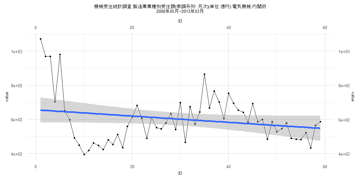
Call:
lm(formula = value ~ ID)

Residuals:
    Min      1Q  Median      3Q     Max
-243.45  -78.36   -5.61   64.10  416.62

Coefficients:
            Estimate Std. Error t value            Pr(>|t|)
(Intercept)  656.973     37.781   17.39 <0.0000000000000002 ***
ID            -1.840      1.095   -1.68              0.0984 .
---
Signif. codes:  0 '***' 0.001 '**' 0.01 '*' 0.05 '.' 0.1 ' ' 1

Residual standard error: 143.3 on 57 degrees of freedom
Multiple R-squared:  0.04719,   Adjusted R-squared:  0.03047
F-statistic: 2.823 on 1 and 57 DF,  p-value: 0.09839


    Two-sample Kolmogorov-Smirnov test

data:  lm_residuals and rnorm(n = length(lm_residuals), mean = 0, sd = sd(lm_residuals))
D = 0.16949, p-value = 0.3674
alternative hypothesis: two-sided


    Durbin-Watson test

data:  value ~ ID
DW = 0.63309, p-value = 0.0000000001688
alternative hypothesis: true autocorrelation is greater than 0


    studentized Breusch-Pagan test

data:  value ~ ID
BP = 17.095, df = 1, p-value = 0.00003555


    Box-Ljung test

data:  lm_residuals
X-squared = 22.985, df = 1, p-value = 0.000001633
Call:
lm(formula = value ~ ID)

Residuals:
     Min       1Q   Median       3Q      Max
-159.101  -51.637   -9.298   47.920  291.736

Coefficients:
            Estimate Std. Error t value            Pr(>|t|)
(Intercept) 600.7952    20.6586  29.082 <0.0000000000000002 ***
ID           -0.3571     0.4544  -0.786               0.434
---
Signif. codes:  0 '***' 0.001 '**' 0.01 '*' 0.05 '.' 0.1 ' ' 1

Residual standard error: 90.35 on 76 degrees of freedom
Multiple R-squared:  0.00806,   Adjusted R-squared:  -0.004992
F-statistic: 0.6175 on 1 and 76 DF,  p-value: 0.4344


    Two-sample Kolmogorov-Smirnov test

data:  lm_residuals and rnorm(n = length(lm_residuals), mean = 0, sd = sd(lm_residuals))
D = 0.19231, p-value = 0.1118
alternative hypothesis: two-sided


    Durbin-Watson test

data:  value ~ ID
DW = 1.1966, p-value = 0.00006162
alternative hypothesis: true autocorrelation is greater than 0


    studentized Breusch-Pagan test

data:  value ~ ID
BP = 0.057391, df = 1, p-value = 0.8107


    Box-Ljung test

data:  lm_residuals
X-squared = 13.007, df = 1, p-value = 0.0003104