Analysis
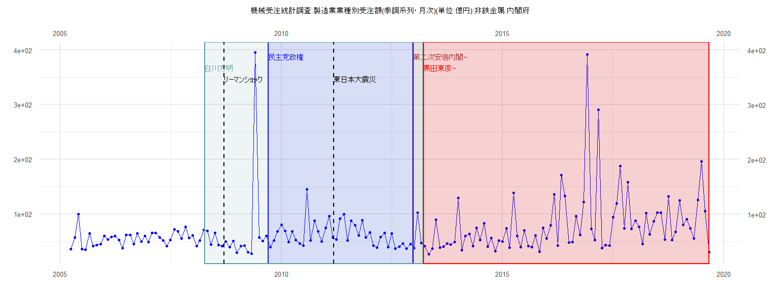
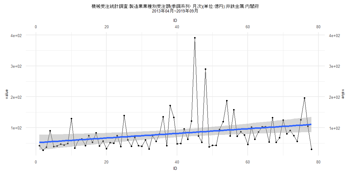
[1] "機械受注統計調査:製造業業種別受注額(季調系列・月次)(単位:億円):非鉄金属:内閣府"
        Jan    Feb    Mar    Apr    May    Jun    Jul    Aug    Sep    Oct    Nov    Dec
2005                       35.87  56.78  99.76  35.96  35.38  64.26  41.10  43.44  44.75
2006  60.09  53.85  57.90  60.11  52.33  37.65  61.77  62.01  45.15  64.87  49.50  59.89
2007  49.23  65.29  65.72  57.05  51.48  41.74  52.50  72.10  68.66  55.66  76.35  56.72
2008  60.87  41.73  51.53  71.47  69.47  43.85  65.55  43.04  41.75  50.21  40.06  50.61
2009  29.29  41.05  42.01  30.59  27.41 395.33  56.96  50.44  60.17  39.41  51.92  67.94
2010  80.86  68.83  49.21  68.32  52.48  45.71  42.51 145.06  52.14  88.27  68.81  50.24
2011  74.38  96.08  57.21  53.08  91.77  99.40  52.01  87.92  79.50  61.38  88.98  57.28
2012  66.15  42.27  38.45  58.40  65.69  39.93  64.56  37.26  40.56  45.92  37.25  45.43
2013  37.60 102.76  47.28  41.34  27.08  36.82  90.00  38.80  40.34  46.31  43.94  48.95
2014 129.63  33.69  59.91  63.60  41.92  74.62  52.59  83.38  40.78  56.68  31.89  51.63
2015  50.00  74.27  38.98 139.18  60.16  39.71  69.84  41.47  39.80  60.60  31.06  74.56
2016  55.76  79.69 135.54  42.18 171.56 133.45  47.91  48.44  96.31  62.30 121.87 391.40
2017  72.93  52.26 290.42  38.18  43.22  42.47  94.48 119.39 187.63  73.52 158.07  72.65
2018  87.55  76.30  45.51 101.95  62.86  86.43 102.40 103.03  53.91 132.73  52.34  66.99
2019 124.98  80.02  90.88  74.24  55.59 125.87 196.57 105.02  29.93
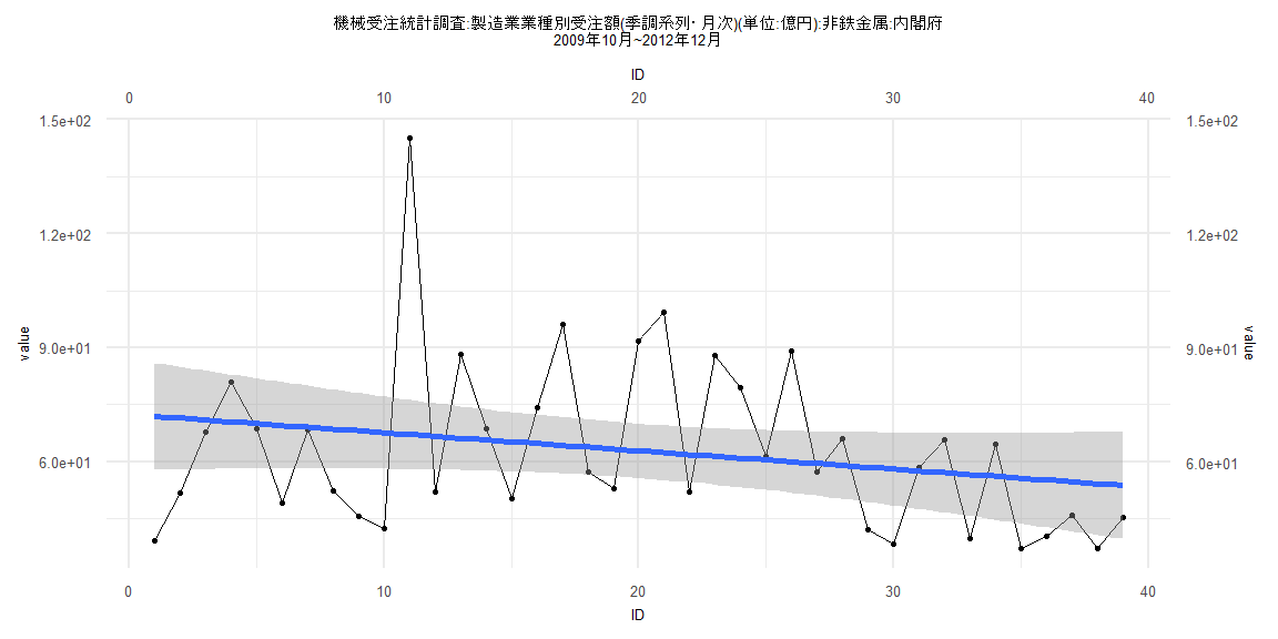
Call:
lm(formula = value ~ ID)

Residuals:
    Min      1Q  Median      3Q     Max
-32.555 -16.228  -3.069   9.060  77.873

Coefficients:
            Estimate Std. Error t value         Pr(>|t|)
(Intercept)  72.4425     7.1879  10.078 0.00000000000371 ***
ID           -0.4778     0.3132  -1.526            0.136
---
Signif. codes:  0 '***' 0.001 '**' 0.01 '*' 0.05 '.' 0.1 ' ' 1

Residual standard error: 22.01 on 37 degrees of freedom
Multiple R-squared:  0.05917,   Adjusted R-squared:  0.03375
F-statistic: 2.327 on 1 and 37 DF,  p-value: 0.1356


    Two-sample Kolmogorov-Smirnov test

data:  lm_residuals and rnorm(n = length(lm_residuals), mean = 0, sd = sd(lm_residuals))
D = 0.10256, p-value = 0.9885
alternative hypothesis: two-sided


    Durbin-Watson test

data:  value ~ ID
DW = 2.0147, p-value = 0.4499
alternative hypothesis: true autocorrelation is greater than 0


    studentized Breusch-Pagan test

data:  value ~ ID
BP = 1.2299, df = 1, p-value = 0.2674


    Box-Ljung test

data:  lm_residuals
X-squared = 0.063563, df = 1, p-value = 0.801
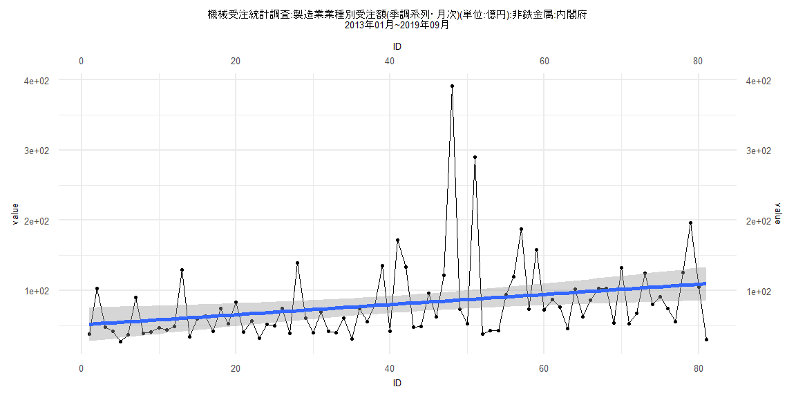
Call:
lm(formula = value ~ ID)

Residuals:
    Min      1Q  Median      3Q     Max
-79.574 -31.492 -13.444   4.734 305.749

Coefficients:
            Estimate Std. Error t value  Pr(>|t|)
(Intercept)  50.9562    12.2575   4.157 0.0000811 ***
ID            0.7228     0.2597   2.783   0.00673 **
---
Signif. codes:  0 '***' 0.001 '**' 0.01 '*' 0.05 '.' 0.1 ' ' 1

Residual standard error: 54.65 on 79 degrees of freedom
Multiple R-squared:  0.0893,    Adjusted R-squared:  0.07777
F-statistic: 7.746 on 1 and 79 DF,  p-value: 0.006731


    Two-sample Kolmogorov-Smirnov test

data:  lm_residuals and rnorm(n = length(lm_residuals), mean = 0, sd = sd(lm_residuals))
D = 0.22222, p-value = 0.03633
alternative hypothesis: two-sided


    Durbin-Watson test

data:  value ~ ID
DW = 2.0639, p-value = 0.5688
alternative hypothesis: true autocorrelation is greater than 0


    studentized Breusch-Pagan test

data:  value ~ ID
BP = 0.63918, df = 1, p-value = 0.424


    Box-Ljung test

data:  lm_residuals
X-squared = 0.1761, df = 1, p-value = 0.6747
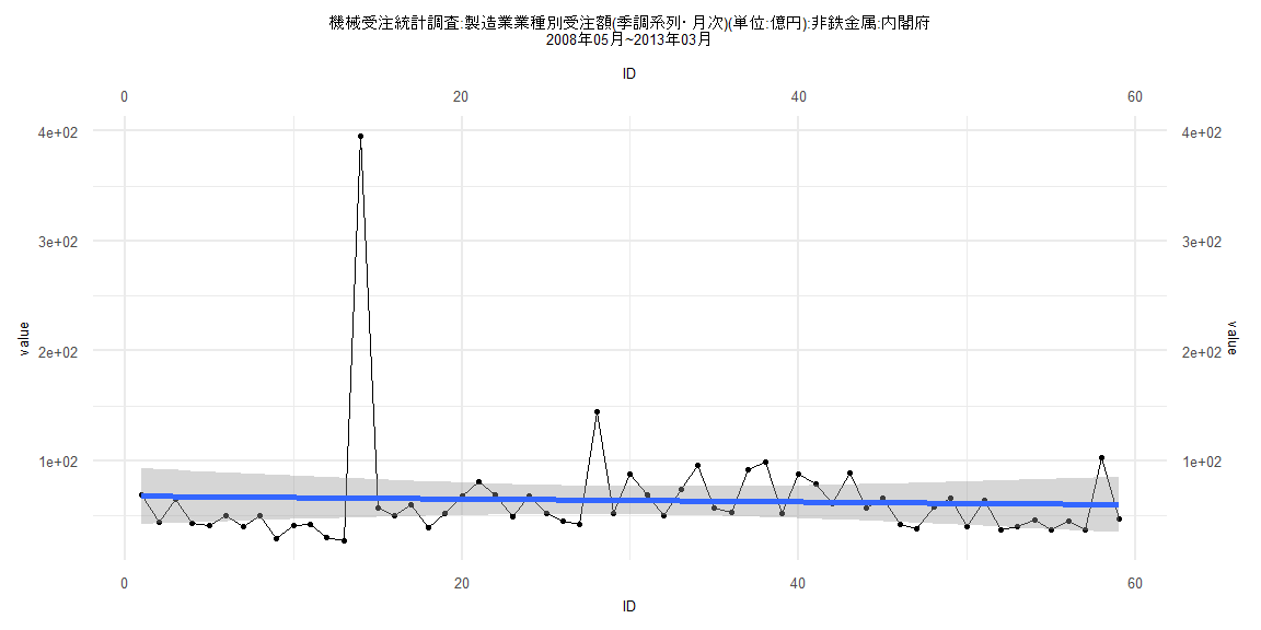
Call:
lm(formula = value ~ ID)

Residuals:
   Min     1Q Median     3Q    Max
-38.87 -21.69 -12.03   3.92 329.18

Coefficients:
            Estimate Std. Error t value   Pr(>|t|)
(Intercept)  68.0010    12.9904   5.235 0.00000247 ***
ID           -0.1322     0.3766  -0.351      0.727
---
Signif. codes:  0 '***' 0.001 '**' 0.01 '*' 0.05 '.' 0.1 ' ' 1

Residual standard error: 49.26 on 57 degrees of freedom
Multiple R-squared:  0.002159,  Adjusted R-squared:  -0.01535
F-statistic: 0.1233 on 1 and 57 DF,  p-value: 0.7268


    Two-sample Kolmogorov-Smirnov test

data:  lm_residuals and rnorm(n = length(lm_residuals), mean = 0, sd = sd(lm_residuals))
D = 0.27119, p-value = 0.02566
alternative hypothesis: two-sided


    Durbin-Watson test

data:  value ~ ID
DW = 2.1444, p-value = 0.6634
alternative hypothesis: true autocorrelation is greater than 0


    studentized Breusch-Pagan test

data:  value ~ ID
BP = 0.9368, df = 1, p-value = 0.3331


    Box-Ljung test

data:  lm_residuals
X-squared = 0.32914, df = 1, p-value = 0.5662
Call:
lm(formula = value ~ ID)

Residuals:
    Min      1Q  Median      3Q     Max
-80.376 -31.581 -13.428   5.181 305.969

Coefficients:
            Estimate Std. Error t value Pr(>|t|)
(Intercept)  51.5113    12.6634   4.068 0.000115 ***
ID            0.7538     0.2785   2.706 0.008396 **
---
Signif. codes:  0 '***' 0.001 '**' 0.01 '*' 0.05 '.' 0.1 ' ' 1

Residual standard error: 55.38 on 76 degrees of freedom
Multiple R-squared:  0.0879,    Adjusted R-squared:  0.0759
F-statistic: 7.324 on 1 and 76 DF,  p-value: 0.008396


    Two-sample Kolmogorov-Smirnov test

data:  lm_residuals and rnorm(n = length(lm_residuals), mean = 0, sd = sd(lm_residuals))
D = 0.23077, p-value = 0.03108
alternative hypothesis: two-sided


    Durbin-Watson test

data:  value ~ ID
DW = 2.0573, p-value = 0.5543
alternative hypothesis: true autocorrelation is greater than 0


    studentized Breusch-Pagan test

data:  value ~ ID
BP = 0.53584, df = 1, p-value = 0.4642


    Box-Ljung test

data:  lm_residuals
X-squared = 0.14815, df = 1, p-value = 0.7003