Analysis
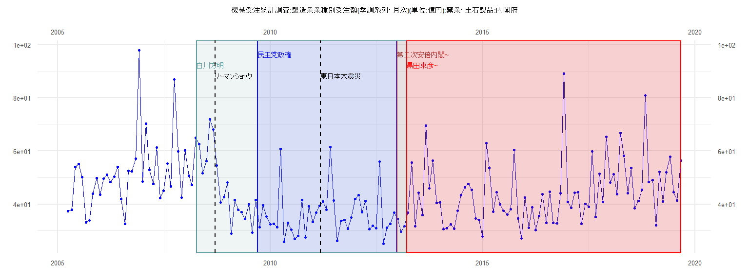
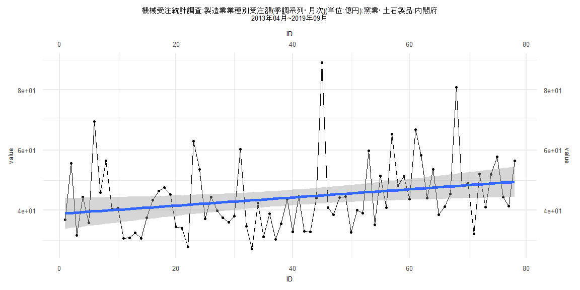
[1] "機械受注統計調査:製造業業種別受注額(季調系列・月次)(単位:億円):窯業・土石製品:内閣府"
       Jan   Feb   Mar   Apr   May   Jun   Jul   Aug   Sep   Oct   Nov   Dec
2005                   37.37 37.99 53.94 55.03 50.26 33.21 33.95 43.96 49.89
2006 43.63 49.60 51.07 48.36 50.42 54.06 41.97 32.66 52.60 52.45 57.03 97.84
2007 48.55 70.22 52.95 47.54 61.31 42.24 45.01 55.27 46.68 86.89 59.84 42.44
2008 60.20 50.76 47.33 65.06 62.64 51.69 56.14 71.90 68.03 54.57 40.76 42.75
2009 48.16 28.98 41.63 37.97 36.95 34.38 39.88 29.44 41.67 31.40 39.58 35.40
2010 32.48 32.70 31.40 60.77 25.79 32.97 30.40 26.96 28.04 41.65 27.52 39.14
2011 33.30 36.93 39.43 40.95 37.90 61.51 41.36 26.30 33.76 34.11 30.86 35.04
2012 42.01 43.35 37.04 41.29 30.59 31.82 31.03 56.01 25.23 31.17 32.57 36.80
2013 34.49 29.77 31.71 36.83 55.69 31.64 44.36 35.86 69.53 45.91 56.39 40.42
2014 40.66 30.65 30.95 32.48 30.73 37.60 43.45 46.40 47.57 45.34 34.61 34.08
2015 27.83 63.03 53.56 37.23 44.43 39.88 37.49 36.05 38.09 60.33 34.73 27.20
2016 42.48 31.22 38.89 30.32 35.63 43.73 32.94 44.65 33.02 32.85 44.17 89.09
2017 40.91 38.61 44.32 44.52 32.65 40.06 39.12 59.81 35.25 51.52 40.85 65.26
2018 48.24 51.23 43.78 66.77 58.30 44.11 53.65 38.53 41.19 45.37 80.92 48.27
2019 49.12 32.14 52.13 41.04 51.99 57.82 44.45 41.45 56.46
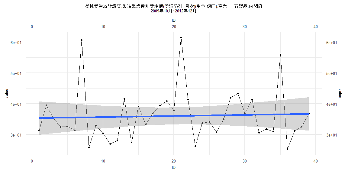
Call:
lm(formula = value ~ ID)

Residuals:
    Min      1Q  Median      3Q     Max
-11.400  -5.365  -2.447   3.792  25.409

Coefficients:
            Estimate Std. Error t value            Pr(>|t|)
(Intercept) 35.35953    2.78401  12.701 0.00000000000000465 ***
ID           0.03531    0.12131   0.291               0.773
---
Signif. codes:  0 '***' 0.001 '**' 0.01 '*' 0.05 '.' 0.1 ' ' 1

Residual standard error: 8.526 on 37 degrees of freedom
Multiple R-squared:  0.002284,  Adjusted R-squared:  -0.02468
F-statistic: 0.0847 on 1 and 37 DF,  p-value: 0.7727


    Two-sample Kolmogorov-Smirnov test

data:  lm_residuals and rnorm(n = length(lm_residuals), mean = 0, sd = sd(lm_residuals))
D = 0.20513, p-value = 0.3888
alternative hypothesis: two-sided


    Durbin-Watson test

data:  value ~ ID
DW = 2.2165, p-value = 0.6956
alternative hypothesis: true autocorrelation is greater than 0


    studentized Breusch-Pagan test

data:  value ~ ID
BP = 0.0089446, df = 1, p-value = 0.9247


    Box-Ljung test

data:  lm_residuals
X-squared = 0.52065, df = 1, p-value = 0.4706
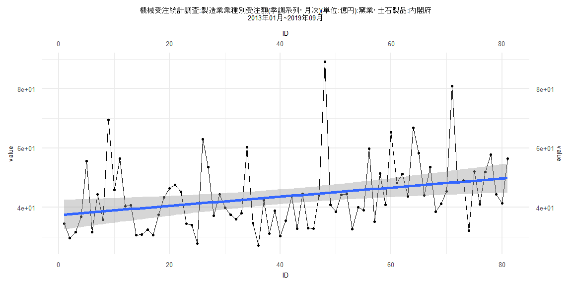
Call:
lm(formula = value ~ ID)

Residuals:
    Min      1Q  Median      3Q     Max
-16.704  -7.084  -2.847   4.483  44.240

Coefficients:
            Estimate Std. Error t value             Pr(>|t|)
(Intercept) 37.47800    2.51874  14.880 < 0.0000000000000002 ***
ID           0.15359    0.05337   2.878              0.00514 **
---
Signif. codes:  0 '***' 0.001 '**' 0.01 '*' 0.05 '.' 0.1 ' ' 1

Residual standard error: 11.23 on 79 degrees of freedom
Multiple R-squared:  0.09491,   Adjusted R-squared:  0.08345
F-statistic: 8.284 on 1 and 79 DF,  p-value: 0.005143


    Two-sample Kolmogorov-Smirnov test

data:  lm_residuals and rnorm(n = length(lm_residuals), mean = 0, sd = sd(lm_residuals))
D = 0.14815, p-value = 0.338
alternative hypothesis: two-sided


    Durbin-Watson test

data:  value ~ ID
DW = 1.948, p-value = 0.3632
alternative hypothesis: true autocorrelation is greater than 0


    studentized Breusch-Pagan test

data:  value ~ ID
BP = 0.046587, df = 1, p-value = 0.8291


    Box-Ljung test

data:  lm_residuals
X-squared = 0.045809, df = 1, p-value = 0.8305
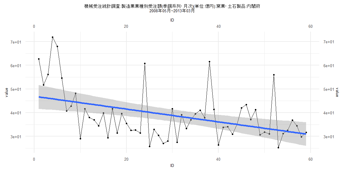
Call:
lm(formula = value ~ ID)

Residuals:
    Min      1Q  Median      3Q     Max
-15.245  -6.695  -1.470   3.711  26.052

Coefficients:
            Estimate Std. Error t value             Pr(>|t|)
(Intercept) 46.93009    2.57922  18.195 < 0.0000000000000002 ***
ID          -0.27051    0.07477  -3.618             0.000631 ***
---
Signif. codes:  0 '***' 0.001 '**' 0.01 '*' 0.05 '.' 0.1 ' ' 1

Residual standard error: 9.78 on 57 degrees of freedom
Multiple R-squared:  0.1868,    Adjusted R-squared:  0.1725
F-statistic: 13.09 on 1 and 57 DF,  p-value: 0.0006309


    Two-sample Kolmogorov-Smirnov test

data:  lm_residuals and rnorm(n = length(lm_residuals), mean = 0, sd = sd(lm_residuals))
D = 0.23729, p-value = 0.07193
alternative hypothesis: two-sided


    Durbin-Watson test

data:  value ~ ID
DW = 1.4184, p-value = 0.007458
alternative hypothesis: true autocorrelation is greater than 0


    studentized Breusch-Pagan test

data:  value ~ ID
BP = 3.5004, df = 1, p-value = 0.06135


    Box-Ljung test

data:  lm_residuals
X-squared = 4.4353, df = 1, p-value = 0.0352
Call:
lm(formula = value ~ ID)

Residuals:
    Min      1Q  Median      3Q     Max
-16.368  -7.634  -2.623   4.804  44.114

Coefficients:
            Estimate Std. Error t value            Pr(>|t|)
(Intercept)  38.8620     2.6008  14.942 <0.0000000000000002 ***
ID            0.1359     0.0572   2.375              0.0201 *
---
Signif. codes:  0 '***' 0.001 '**' 0.01 '*' 0.05 '.' 0.1 ' ' 1

Residual standard error: 11.37 on 76 degrees of freedom
Multiple R-squared:  0.0691,    Adjusted R-squared:  0.05685
F-statistic: 5.641 on 1 and 76 DF,  p-value: 0.02007


    Two-sample Kolmogorov-Smirnov test

data:  lm_residuals and rnorm(n = length(lm_residuals), mean = 0, sd = sd(lm_residuals))
D = 0.12821, p-value = 0.546
alternative hypothesis: two-sided


    Durbin-Watson test

data:  value ~ ID
DW = 1.9684, p-value = 0.3984
alternative hypothesis: true autocorrelation is greater than 0


    studentized Breusch-Pagan test

data:  value ~ ID
BP = 0.0067398, df = 1, p-value = 0.9346


    Box-Ljung test

data:  lm_residuals
X-squared = 0.01384, df = 1, p-value = 0.9063