Analysis
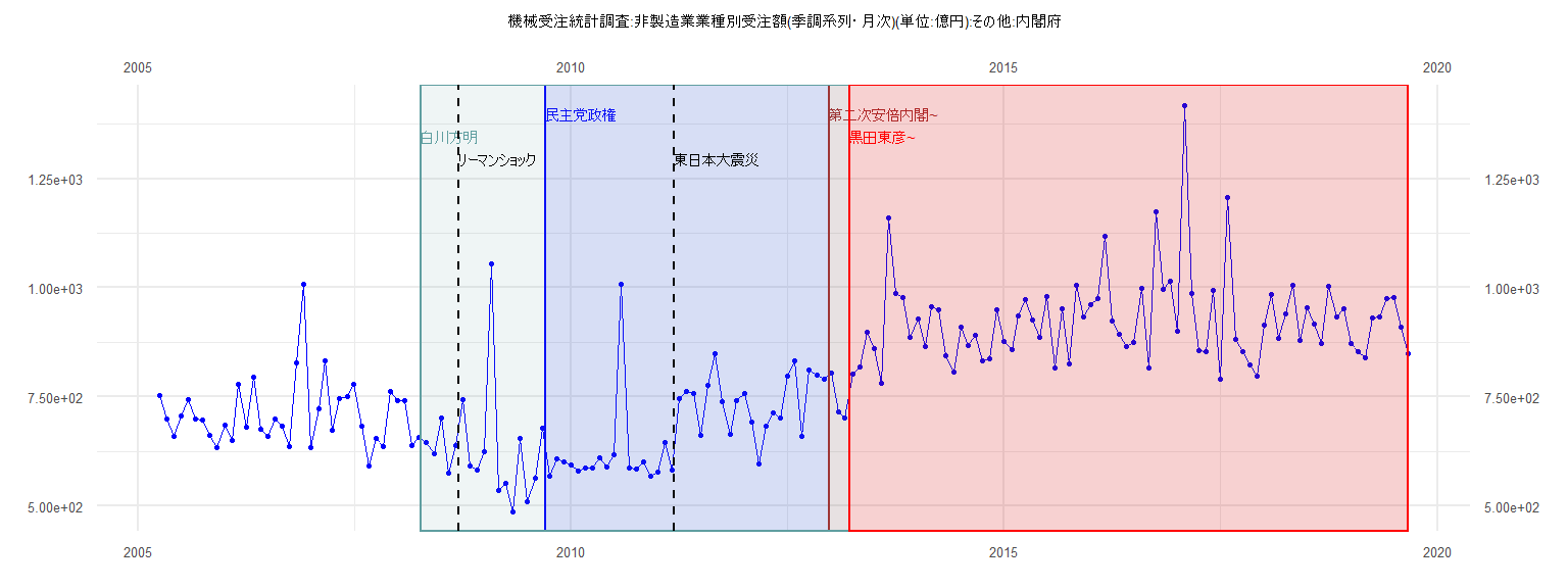
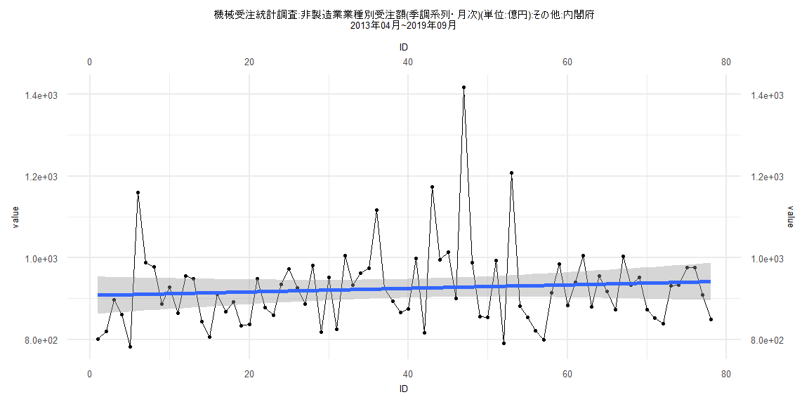
[1] "機械受注統計調査:非製造業業種別受注額(季調系列・月次)(単位:億円):その他:内閣府"
         Jan     Feb     Mar     Apr     May     Jun     Jul     Aug     Sep     Oct     Nov     Dec
2005                          752.04  700.46  660.46  707.47  743.98  699.96  696.47  661.24  632.91
2006  685.05  650.06  779.90  679.53  795.84  675.38  658.85  699.99  682.99  636.71  827.14 1009.01
2007  634.97  723.79  833.37  674.03  747.02  750.77  777.70  682.07  592.66  654.86  636.03  763.37
2008  741.21  741.74  638.15  657.49  646.32  619.97  700.89  576.09  638.27  744.26  590.60  582.02
2009  623.31 1055.96  535.69  552.60  487.51  655.91  510.03  564.24  677.36  569.43  608.70  600.37
2010  593.75  579.97  586.78  586.44  610.16  588.78  618.06 1008.49  586.50  583.58  600.99  569.16
2011  577.18  645.54  581.41  746.73  762.30  758.30  662.49  776.58  848.38  738.72  663.09  741.42
2012  758.08  691.72  597.37  682.85  714.48  700.73  797.50  832.62  658.84  810.68  800.79  790.50
2013  803.61  716.07  701.90  801.33  819.58  897.05  860.79  782.24 1160.56  988.00  977.29  887.15
2014  928.37  864.30  956.25  949.40  843.55  806.19  910.45  867.23  891.81  833.79  837.15  948.79
2015  877.59  859.45  935.50  973.16  926.50  886.70  981.13  817.34  952.10  825.81 1005.89  933.16
2016  961.77  975.17 1117.58  924.89  893.52  866.36  873.99  998.69  816.04 1173.82  995.50 1014.18
2017  901.26 1417.22  987.99  856.79  854.76  993.97  789.87 1207.94  882.08  853.92  822.21  798.56
2018  915.04  984.66  883.38  940.81 1004.83  879.61  955.25  917.92  872.55 1003.37  933.73  951.85
2019  872.70  852.88  838.67  931.45  933.77  975.78  976.83  908.80  849.79
Call:
lm(formula = value ~ ID)

Residuals:
    Min      1Q  Median      3Q     Max
-136.20  -49.12  -16.92   32.60  371.37

Coefficients:
            Estimate Std. Error t value             Pr(>|t|)
(Intercept)  581.274     28.040  20.730 < 0.0000000000000002 ***
ID             5.077      1.222   4.155             0.000184 ***
---
Signif. codes:  0 '***' 0.001 '**' 0.01 '*' 0.05 '.' 0.1 ' ' 1

Residual standard error: 85.88 on 37 degrees of freedom
Multiple R-squared:  0.3181,    Adjusted R-squared:  0.2997
F-statistic: 17.26 on 1 and 37 DF,  p-value: 0.0001843


    Two-sample Kolmogorov-Smirnov test

data:  lm_residuals and rnorm(n = length(lm_residuals), mean = 0, sd = sd(lm_residuals))
D = 0.20513, p-value = 0.3888
alternative hypothesis: two-sided


    Durbin-Watson test

data:  value ~ ID
DW = 1.8623, p-value = 0.2719
alternative hypothesis: true autocorrelation is greater than 0


    studentized Breusch-Pagan test

data:  value ~ ID
BP = 0.22179, df = 1, p-value = 0.6377


    Box-Ljung test

data:  lm_residuals
X-squared = 0.19524, df = 1, p-value = 0.6586
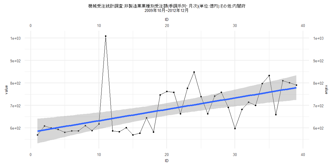
Call:
lm(formula = value ~ ID)

Residuals:
    Min      1Q  Median      3Q     Max
-183.14  -67.80  -17.16   48.24  491.25

Coefficients:
            Estimate Std. Error t value            Pr(>|t|)
(Intercept) 882.4319    23.4047  37.703 <0.0000000000000002 ***
ID            0.8708     0.4959   1.756               0.083 .
---
Signif. codes:  0 '***' 0.001 '**' 0.01 '*' 0.05 '.' 0.1 ' ' 1

Residual standard error: 104.3 on 79 degrees of freedom
Multiple R-squared:  0.03757,   Adjusted R-squared:  0.02539
F-statistic: 3.084 on 1 and 79 DF,  p-value: 0.08295


    Two-sample Kolmogorov-Smirnov test

data:  lm_residuals and rnorm(n = length(lm_residuals), mean = 0, sd = sd(lm_residuals))
D = 0.18519, p-value = 0.1245
alternative hypothesis: two-sided


    Durbin-Watson test

data:  value ~ ID
DW = 1.8546, p-value = 0.2198
alternative hypothesis: true autocorrelation is greater than 0


    studentized Breusch-Pagan test

data:  value ~ ID
BP = 0.0057715, df = 1, p-value = 0.9394


    Box-Ljung test

data:  lm_residuals
X-squared = 0.33154, df = 1, p-value = 0.5648
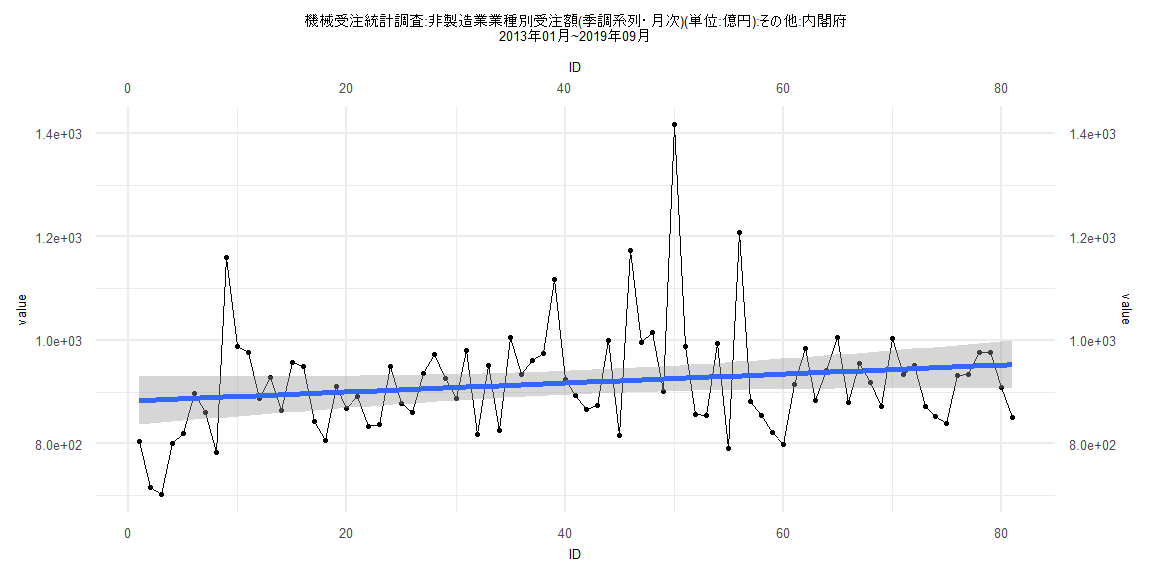
Call:
lm(formula = value ~ ID)

Residuals:
    Min      1Q  Median      3Q     Max
-138.27  -69.68  -30.35   51.04  438.23

Coefficients:
            Estimate Std. Error t value             Pr(>|t|)
(Intercept) 590.9048    26.8538  22.005 < 0.0000000000000002 ***
ID            2.6829     0.7785   3.446              0.00107 **
---
Signif. codes:  0 '***' 0.001 '**' 0.01 '*' 0.05 '.' 0.1 ' ' 1

Residual standard error: 101.8 on 57 degrees of freedom
Multiple R-squared:  0.1724,    Adjusted R-squared:  0.1579
F-statistic: 11.88 on 1 and 57 DF,  p-value: 0.001073


    Two-sample Kolmogorov-Smirnov test

data:  lm_residuals and rnorm(n = length(lm_residuals), mean = 0, sd = sd(lm_residuals))
D = 0.18644, p-value = 0.2582
alternative hypothesis: two-sided


    Durbin-Watson test

data:  value ~ ID
DW = 1.8956, p-value = 0.2945
alternative hypothesis: true autocorrelation is greater than 0


    studentized Breusch-Pagan test

data:  value ~ ID
BP = 1.3256, df = 1, p-value = 0.2496


    Box-Ljung test

data:  lm_residuals
X-squared = 0.14278, df = 1, p-value = 0.7055
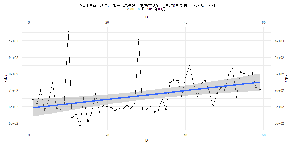
Call:
lm(formula = value ~ ID)

Residuals:
    Min      1Q  Median      3Q     Max
-140.50  -65.05  -15.03   42.17  489.01

Coefficients:
            Estimate Std. Error t value            Pr(>|t|)
(Intercept) 907.9015    23.1942  39.143 <0.0000000000000002 ***
ID            0.4320     0.5101   0.847                 0.4
---
Signif. codes:  0 '***' 0.001 '**' 0.01 '*' 0.05 '.' 0.1 ' ' 1

Residual standard error: 101.4 on 76 degrees of freedom
Multiple R-squared:  0.009348,  Adjusted R-squared:  -0.003687
F-statistic: 0.7171 on 1 and 76 DF,  p-value: 0.3997


    Two-sample Kolmogorov-Smirnov test

data:  lm_residuals and rnorm(n = length(lm_residuals), mean = 0, sd = sd(lm_residuals))
D = 0.076923, p-value = 0.9766
alternative hypothesis: two-sided


    Durbin-Watson test

data:  value ~ ID
DW = 2.0172, p-value = 0.4836
alternative hypothesis: true autocorrelation is greater than 0


    studentized Breusch-Pagan test

data:  value ~ ID
BP = 0.0095786, df = 1, p-value = 0.922


    Box-Ljung test

data:  lm_residuals
X-squared = 0.036861, df = 1, p-value = 0.8477