Analysis
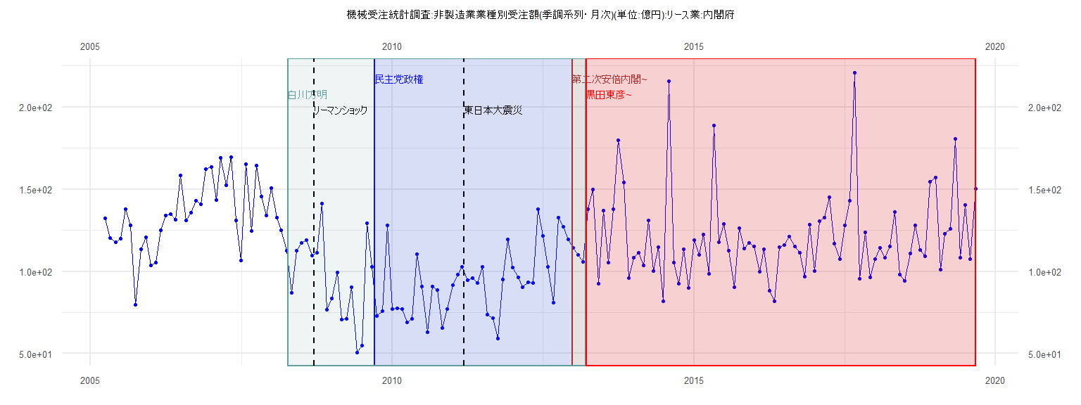
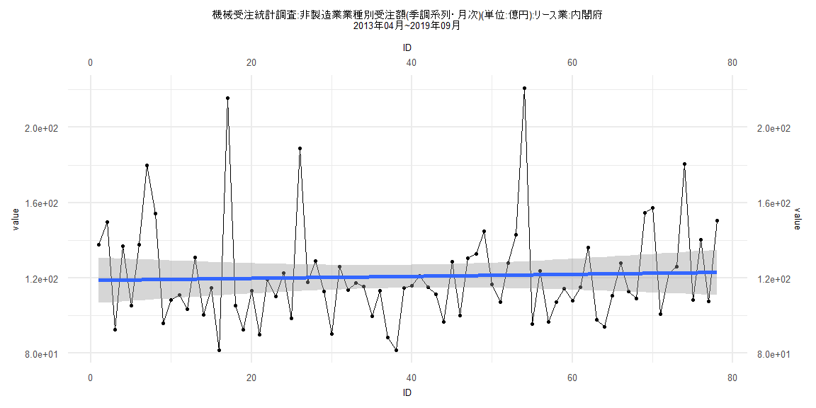
[1] "機械受注統計調査:非製造業業種別受注額(季調系列・月次)(単位:億円):リース業:内閣府"
        Jan    Feb    Mar    Apr    May    Jun    Jul    Aug    Sep    Oct    Nov    Dec
2005                      132.41 120.20 117.57 119.82 138.02 128.12  79.64 113.62 120.59
2006 103.47 105.37 125.11 133.91 135.01 131.37 158.38 131.12 135.54 143.21 140.79 162.40
2007 163.34 143.25 168.95 152.53 169.69 130.90 106.72 165.44 124.61 164.26 145.74 133.92
2008 150.63 132.54 125.00 112.58  87.15 112.78 117.36 118.88 109.70 111.20 141.32  76.73
2009  83.70  99.40  70.88  70.99  90.46  50.81  55.09 129.29 102.65  72.85  75.73 127.85
2010  77.28  77.64  77.18  69.08  71.13 110.45  90.90  63.14  90.98  88.78  65.50  77.09
2011  91.86  98.01 102.75  94.75  96.05  93.07 102.75  73.72  71.47  59.00  95.02 119.66
2012 102.34  96.54  90.53  93.45  92.88 137.88 121.56 102.69  81.08 132.88 127.15 119.44
2013 114.38 109.86 106.00 137.78 149.81  92.65 136.83 105.51 137.75 179.88 154.15  95.92
2014 108.25 111.19 103.47 130.88 100.44 114.86  81.70 215.54 105.27  92.57 113.30  89.98
2015 119.20 110.19 122.51  98.64 188.84 117.87 128.93 112.73  90.41 126.13 113.76 117.28
2016 115.41  99.70 113.38  88.35  81.83 114.82 116.04 121.17 115.06 111.31  96.67 128.65
2017 100.19 130.41 132.83 144.94 116.73 107.41 127.95 143.05 220.83  95.45 123.75  96.55
2018 107.30 114.26 108.17 115.07 136.15  98.00  94.09 110.75 127.86 112.88 109.31 154.68
2019 157.29 100.90 122.77 126.08 180.79 108.40 140.23 107.70 150.34
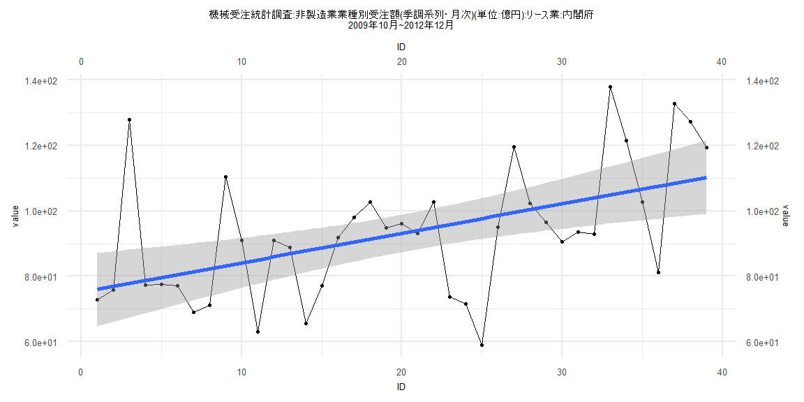
Call:
lm(formula = value ~ ID)

Residuals:
    Min      1Q  Median      3Q     Max
-38.642 -11.126  -1.161   7.700  50.057

Coefficients:
            Estimate Std. Error t value          Pr(>|t|)
(Intercept)  75.0863     5.7502  13.058 0.000000000000002 ***
ID            0.9022     0.2506   3.601          0.000926 ***
---
Signif. codes:  0 '***' 0.001 '**' 0.01 '*' 0.05 '.' 0.1 ' ' 1

Residual standard error: 17.61 on 37 degrees of freedom
Multiple R-squared:  0.2595,    Adjusted R-squared:  0.2395
F-statistic: 12.97 on 1 and 37 DF,  p-value: 0.0009257


    Two-sample Kolmogorov-Smirnov test

data:  lm_residuals and rnorm(n = length(lm_residuals), mean = 0, sd = sd(lm_residuals))
D = 0.15385, p-value = 0.7523
alternative hypothesis: two-sided


    Durbin-Watson test

data:  value ~ ID
DW = 1.6625, p-value = 0.1066
alternative hypothesis: true autocorrelation is greater than 0


    studentized Breusch-Pagan test

data:  value ~ ID
BP = 0.0016307, df = 1, p-value = 0.9678


    Box-Ljung test

data:  lm_residuals
X-squared = 1.1409, df = 1, p-value = 0.2855
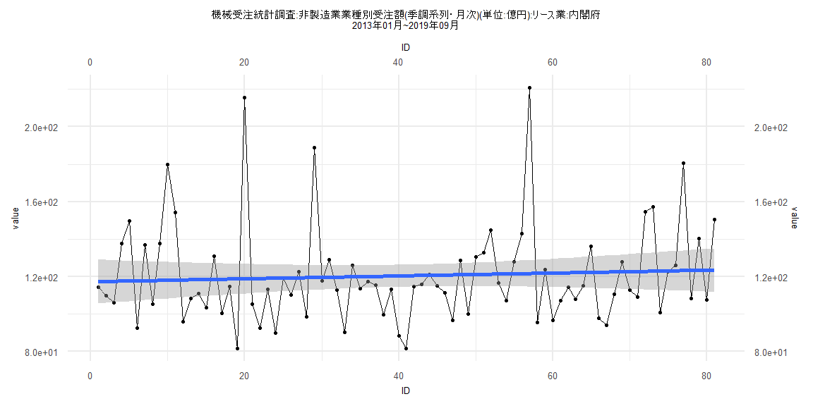
Call:
lm(formula = value ~ ID)

Residuals:
    Min      1Q  Median      3Q     Max
-38.663 -14.932  -5.812   9.204  99.109

Coefficients:
             Estimate Std. Error t value            Pr(>|t|)
(Intercept) 117.34732    5.94760  19.730 <0.0000000000000002 ***
ID            0.07673    0.12601   0.609               0.544
---
Signif. codes:  0 '***' 0.001 '**' 0.01 '*' 0.05 '.' 0.1 ' ' 1

Residual standard error: 26.52 on 79 degrees of freedom
Multiple R-squared:  0.004672,  Adjusted R-squared:  -0.007928
F-statistic: 0.3708 on 1 and 79 DF,  p-value: 0.5443


    Two-sample Kolmogorov-Smirnov test

data:  lm_residuals and rnorm(n = length(lm_residuals), mean = 0, sd = sd(lm_residuals))
D = 0.16049, p-value = 0.2488
alternative hypothesis: two-sided


    Durbin-Watson test

data:  value ~ ID
DW = 2.1041, p-value = 0.6388
alternative hypothesis: true autocorrelation is greater than 0


    studentized Breusch-Pagan test

data:  value ~ ID
BP = 0.096036, df = 1, p-value = 0.7566


    Box-Ljung test

data:  lm_residuals
X-squared = 0.28836, df = 1, p-value = 0.5913
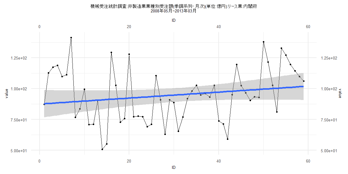
Call:
lm(formula = value ~ ID)

Residuals:
    Min      1Q  Median      3Q     Max
-40.083 -16.129  -2.084  14.878  52.118

Coefficients:
            Estimate Std. Error t value            Pr(>|t|)
(Intercept)  87.5103     5.6172  15.579 <0.0000000000000002 ***
ID            0.2416     0.1628   1.484               0.143
---
Signif. codes:  0 '***' 0.001 '**' 0.01 '*' 0.05 '.' 0.1 ' ' 1

Residual standard error: 21.3 on 57 degrees of freedom
Multiple R-squared:  0.03718,   Adjusted R-squared:  0.02029
F-statistic: 2.201 on 1 and 57 DF,  p-value: 0.1434


    Two-sample Kolmogorov-Smirnov test

data:  lm_residuals and rnorm(n = length(lm_residuals), mean = 0, sd = sd(lm_residuals))
D = 0.10169, p-value = 0.9239
alternative hypothesis: two-sided


    Durbin-Watson test

data:  value ~ ID
DW = 1.3617, p-value = 0.00379
alternative hypothesis: true autocorrelation is greater than 0


    studentized Breusch-Pagan test

data:  value ~ ID
BP = 3.037, df = 1, p-value = 0.08139


    Box-Ljung test

data:  lm_residuals
X-squared = 6.3064, df = 1, p-value = 0.01203
Call:
lm(formula = value ~ ID)

Residuals:
    Min      1Q  Median      3Q     Max
-38.983 -15.067  -6.292   8.997  99.151

Coefficients:
             Estimate Std. Error t value            Pr(>|t|)
(Intercept) 118.75513    6.16887  19.251 <0.0000000000000002 ***
ID            0.05414    0.13568   0.399               0.691
---
Signif. codes:  0 '***' 0.001 '**' 0.01 '*' 0.05 '.' 0.1 ' ' 1

Residual standard error: 26.98 on 76 degrees of freedom
Multiple R-squared:  0.002091,  Adjusted R-squared:  -0.01104
F-statistic: 0.1592 on 1 and 76 DF,  p-value: 0.691


    Two-sample Kolmogorov-Smirnov test

data:  lm_residuals and rnorm(n = length(lm_residuals), mean = 0, sd = sd(lm_residuals))
D = 0.17949, p-value = 0.1624
alternative hypothesis: two-sided


    Durbin-Watson test

data:  value ~ ID
DW = 2.0939, p-value = 0.6176
alternative hypothesis: true autocorrelation is greater than 0


    studentized Breusch-Pagan test

data:  value ~ ID
BP = 0.28027, df = 1, p-value = 0.5965


    Box-Ljung test

data:  lm_residuals
X-squared = 0.26318, df = 1, p-value = 0.6079