Analysis
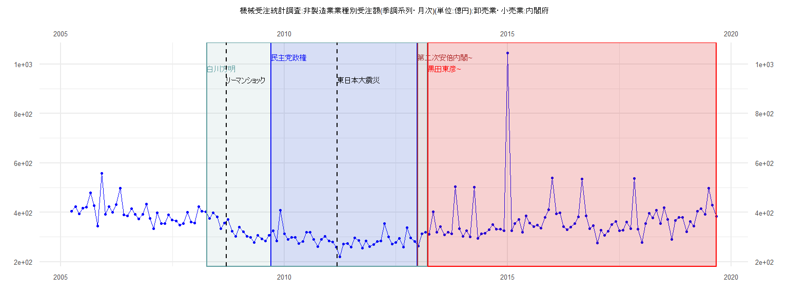
[1] "機械受注統計調査:非製造業業種別受注額(季調系列・月次)(単位:億円):卸売業・小売業:内閣府"
         Jan     Feb     Mar     Apr     May     Jun     Jul     Aug     Sep     Oct     Nov     Dec
2005                          404.10  422.27  393.09  416.33  421.54  480.12  426.77  344.89  558.32
2006  391.20  423.65  401.33  431.21  498.30  389.36  386.15  415.80  391.57  374.08  392.46  433.34
2007  376.00  333.83  397.91  354.12  355.18  390.72  370.09  365.46  348.72  354.72  400.59  359.93
2008  357.73  423.97  403.82  403.31  376.12  397.70  381.53  334.21  356.65  372.23  322.99  303.61
2009  340.01  322.50  302.43  298.55  277.36  307.19  291.92  283.72  306.32  326.35  284.57  408.21
2010  313.88  290.52  298.85  298.18  273.96  282.92  319.76  319.24  290.18  261.63  290.37  301.86
2011  283.20  280.67  259.47  220.85  272.57  273.11  258.54  296.81  285.51  255.67  283.67  260.55
2012  270.53  282.62  283.38  355.64  300.29  271.48  277.96  294.79  259.77  338.76  296.72  283.14
2013  262.94  314.19  319.55  311.26  403.21  319.65  343.20  308.36  318.80  312.64  503.20  333.82
2014  302.04  326.53  299.89  502.24  295.20  312.54  315.33  329.59  350.24  332.81  332.65  325.54
2015 1045.09  326.36  354.57  371.81  318.68  386.55  356.25  342.21  348.40  336.38  379.27  411.02
2016  539.16  393.14  397.85  341.53  330.22  340.28  354.20  381.45  535.43  386.42  333.39  346.80
2017  276.21  327.83  306.66  323.27  350.51  363.50  326.32  328.28  360.20  334.56  536.88  331.07
2018  278.00  354.02  395.86  377.78  407.59  353.82  418.10  372.16  289.86  366.75  379.22  380.49
2019  322.49  362.41  344.85  403.55  413.91  392.11  498.81  429.45  384.21
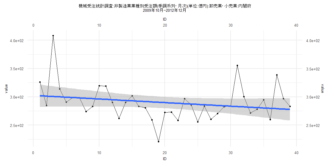
Call:
lm(formula = value ~ ID)

Residuals:
    Min      1Q  Median      3Q     Max
-69.686 -16.447  -3.073  11.325 107.538

Coefficients:
            Estimate Std. Error t value            Pr(>|t|)
(Intercept) 302.5723    10.1019  29.952 <0.0000000000000002 ***
ID           -0.6335     0.4402  -1.439               0.158
---
Signif. codes:  0 '***' 0.001 '**' 0.01 '*' 0.05 '.' 0.1 ' ' 1

Residual standard error: 30.94 on 37 degrees of freedom
Multiple R-squared:  0.05301,   Adjusted R-squared:  0.02742
F-statistic: 2.071 on 1 and 37 DF,  p-value: 0.1585


    Two-sample Kolmogorov-Smirnov test

data:  lm_residuals and rnorm(n = length(lm_residuals), mean = 0, sd = sd(lm_residuals))
D = 0.20513, p-value = 0.3888
alternative hypothesis: two-sided


    Durbin-Watson test

data:  value ~ ID
DW = 1.6726, p-value = 0.1128
alternative hypothesis: true autocorrelation is greater than 0


    studentized Breusch-Pagan test

data:  value ~ ID
BP = 0.45055, df = 1, p-value = 0.5021


    Box-Ljung test

data:  lm_residuals
X-squared = 1.0094, df = 1, p-value = 0.3151
Call:
lm(formula = value ~ ID)

Residuals:
   Min     1Q Median     3Q    Max
-98.96 -40.67 -22.94  11.95 683.93

Coefficients:
            Estimate Std. Error t value            Pr(>|t|)
(Intercept) 350.1785    21.3999  16.364 <0.0000000000000002 ***
ID            0.4391     0.4534   0.968               0.336
---
Signif. codes:  0 '***' 0.001 '**' 0.01 '*' 0.05 '.' 0.1 ' ' 1

Residual standard error: 95.41 on 79 degrees of freedom
Multiple R-squared:  0.01173,   Adjusted R-squared:  -0.0007785
F-statistic: 0.9378 on 1 and 79 DF,  p-value: 0.3358


    Two-sample Kolmogorov-Smirnov test

data:  lm_residuals and rnorm(n = length(lm_residuals), mean = 0, sd = sd(lm_residuals))
D = 0.20988, p-value = 0.05619
alternative hypothesis: two-sided


    Durbin-Watson test

data:  value ~ ID
DW = 2.0401, p-value = 0.5264
alternative hypothesis: true autocorrelation is greater than 0


    studentized Breusch-Pagan test

data:  value ~ ID
BP = 0.52258, df = 1, p-value = 0.4697


    Box-Ljung test

data:  lm_residuals
X-squared = 0.054265, df = 1, p-value = 0.8158
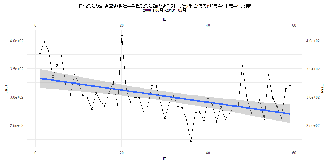
Call:
lm(formula = value ~ ID)

Residuals:
   Min     1Q Median     3Q    Max
-73.99 -20.38  -8.23  15.48  96.08

Coefficients:
            Estimate Std. Error t value             Pr(>|t|)
(Intercept) 333.7364     8.4434  39.526 < 0.0000000000000002 ***
ID           -1.0805     0.2448  -4.415            0.0000457 ***
---
Signif. codes:  0 '***' 0.001 '**' 0.01 '*' 0.05 '.' 0.1 ' ' 1

Residual standard error: 32.02 on 57 degrees of freedom
Multiple R-squared:  0.2548,    Adjusted R-squared:  0.2417
F-statistic: 19.49 on 1 and 57 DF,  p-value: 0.00004565


    Two-sample Kolmogorov-Smirnov test

data:  lm_residuals and rnorm(n = length(lm_residuals), mean = 0, sd = sd(lm_residuals))
D = 0.20339, p-value = 0.1748
alternative hypothesis: two-sided


    Durbin-Watson test

data:  value ~ ID
DW = 1.2563, p-value = 0.0009062
alternative hypothesis: true autocorrelation is greater than 0


    studentized Breusch-Pagan test

data:  value ~ ID
BP = 0.14683, df = 1, p-value = 0.7016


    Box-Ljung test

data:  lm_residuals
X-squared = 6.9506, df = 1, p-value = 0.008379
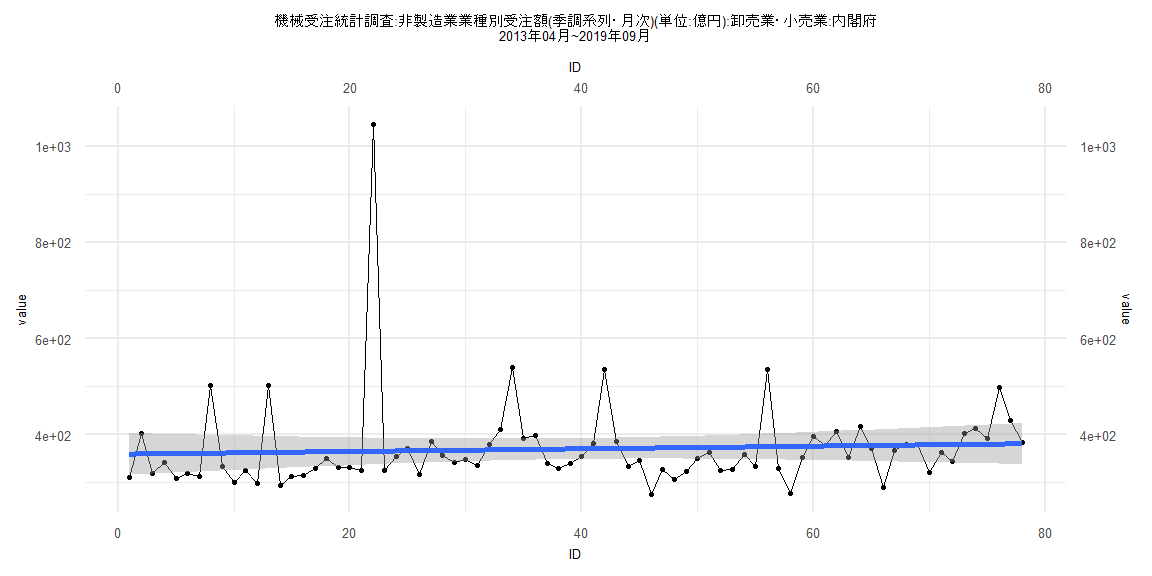
Call:
lm(formula = value ~ ID)

Residuals:
   Min     1Q Median     3Q    Max
-97.98 -42.33 -22.74  11.19 679.10

Coefficients:
            Estimate Std. Error t value            Pr(>|t|)
(Intercept) 359.8892    22.0646  16.311 <0.0000000000000002 ***
ID            0.2774     0.4853   0.572               0.569
---
Signif. codes:  0 '***' 0.001 '**' 0.01 '*' 0.05 '.' 0.1 ' ' 1

Residual standard error: 96.5 on 76 degrees of freedom
Multiple R-squared:  0.00428,   Adjusted R-squared:  -0.008822
F-statistic: 0.3267 on 1 and 76 DF,  p-value: 0.5693


    Two-sample Kolmogorov-Smirnov test

data:  lm_residuals and rnorm(n = length(lm_residuals), mean = 0, sd = sd(lm_residuals))
D = 0.21795, p-value = 0.04892
alternative hypothesis: two-sided


    Durbin-Watson test

data:  value ~ ID
DW = 2.0693, p-value = 0.5752
alternative hypothesis: true autocorrelation is greater than 0


    studentized Breusch-Pagan test

data:  value ~ ID
BP = 0.68129, df = 1, p-value = 0.4091


    Box-Ljung test

data:  lm_residuals
X-squared = 0.10695, df = 1, p-value = 0.7436