Analysis
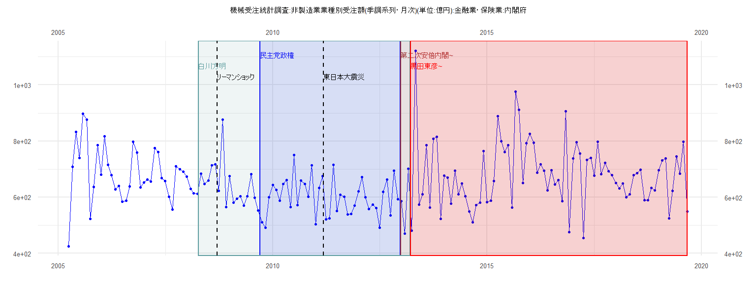
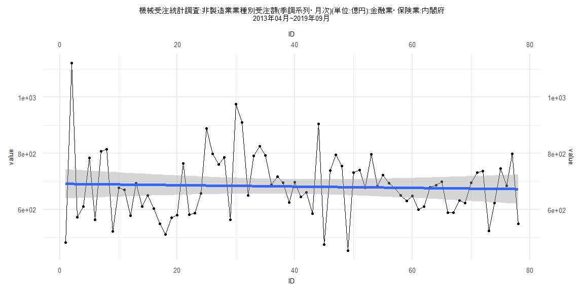
[1] "機械受注統計調査:非製造業業種別受注額(季調系列・月次)(単位:億円):金融業・保険業:内閣府"
         Jan     Feb     Mar     Apr     May     Jun     Jul     Aug     Sep     Oct     Nov     Dec
2005                          425.52  707.73  832.09  740.57  897.73  876.85  522.44  636.85  785.41
2006  681.25  817.40  715.10  679.08  627.99  640.96  584.09  587.41  638.16  798.56  759.74  634.42
2007  651.51  662.90  656.18  774.44  761.37  668.35  658.29  601.48  556.22  710.95  700.04  690.47
2008  672.51  629.98  614.06  611.82  684.06  647.99  659.56  712.78  716.57  622.74  876.40  565.62
2009  674.97  580.87  594.81  602.81  570.86  604.10  682.93  598.55  551.81  511.17  491.63  599.44
2010  643.70  626.07  587.99  647.40  660.61  564.36  750.74  571.64  659.42  646.49  601.77  714.11
2011  502.79  633.68  674.41  520.57  525.24  716.10  550.44  608.57  601.63  538.85  540.86  570.40
2012  621.40  671.38  599.13  557.14  573.58  561.97  491.79  619.92  663.28  534.59  694.30  592.59
2013  586.10  470.23  700.54  481.62 1121.53  573.26  610.41  784.59  563.70  807.60  815.13  522.96
2014  676.68  670.69  577.70  693.74  610.82  649.61  603.58  549.25  510.92  571.49  580.80  764.78
2015  582.35  587.90  657.53  888.04  799.21  760.70  786.24  563.57  976.24  911.13  649.77  792.10
2016  825.30  793.73  687.52  717.48  695.10  624.44  696.57  645.10  661.06  585.40  905.57  476.09
2017  738.92  795.63  755.02  453.65  732.10  739.86  676.90  797.31  682.37  722.21  693.24  678.28
2018  650.03  631.19  649.15  600.54  610.35  678.68  685.85  698.30  588.78  589.05  632.74  623.66
2019  696.25  730.85  737.57  523.77  623.30  745.41  684.31  798.55  549.45
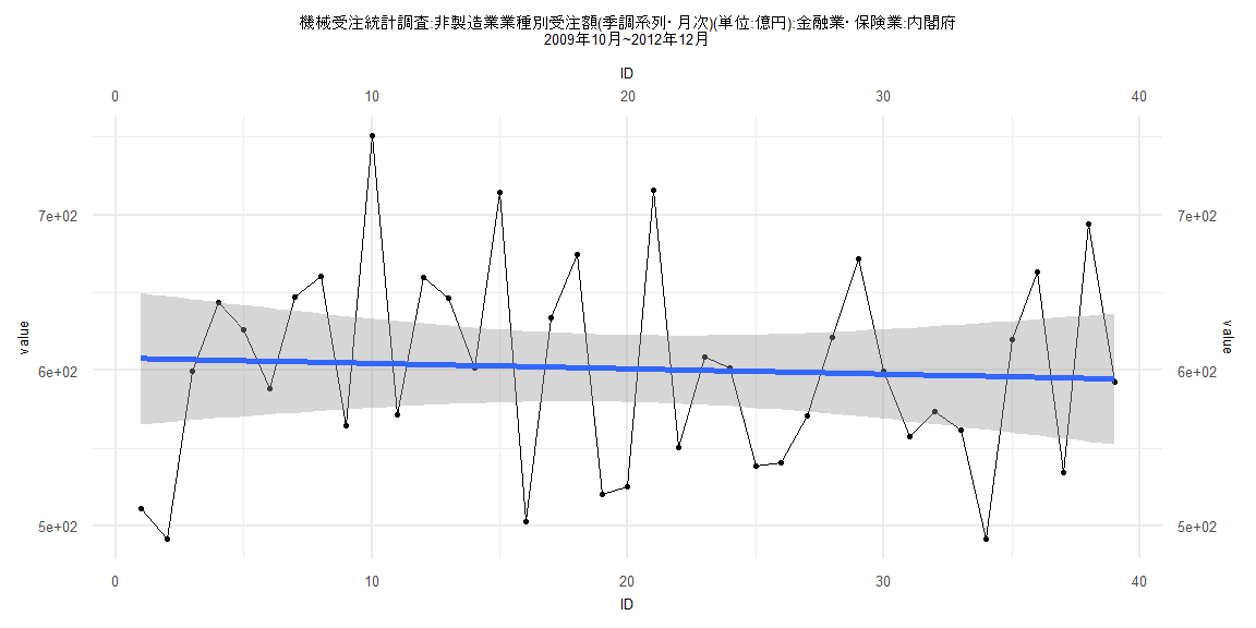
Call:
lm(formula = value ~ ID)

Residuals:
     Min       1Q   Median       3Q      Max
-115.608  -45.201   -1.346   42.455  146.250

Coefficients:
            Estimate Std. Error t value            Pr(>|t|)
(Intercept) 607.9252    21.6181  28.121 <0.0000000000000002 ***
ID           -0.3435     0.9420  -0.365               0.717
---
Signif. codes:  0 '***' 0.001 '**' 0.01 '*' 0.05 '.' 0.1 ' ' 1

Residual standard error: 66.21 on 37 degrees of freedom
Multiple R-squared:  0.003581,  Adjusted R-squared:  -0.02335
F-statistic: 0.133 on 1 and 37 DF,  p-value: 0.7174


    Two-sample Kolmogorov-Smirnov test

data:  lm_residuals and rnorm(n = length(lm_residuals), mean = 0, sd = sd(lm_residuals))
D = 0.076923, p-value = 0.9999
alternative hypothesis: two-sided


    Durbin-Watson test

data:  value ~ ID
DW = 2.2531, p-value = 0.7351
alternative hypothesis: true autocorrelation is greater than 0


    studentized Breusch-Pagan test

data:  value ~ ID
BP = 0.66783, df = 1, p-value = 0.4138


    Box-Ljung test

data:  lm_residuals
X-squared = 1.0139, df = 1, p-value = 0.314
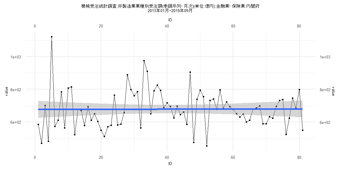
Call:
lm(formula = value ~ ID)

Residuals:
    Min      1Q  Median      3Q     Max
-225.31  -89.99   -1.01   60.82  444.50

Coefficients:
             Estimate Std. Error t value            Pr(>|t|)
(Intercept) 676.82098   26.35587  25.680 <0.0000000000000002 ***
ID            0.04114    0.55841   0.074               0.941
---
Signif. codes:  0 '***' 0.001 '**' 0.01 '*' 0.05 '.' 0.1 ' ' 1

Residual standard error: 117.5 on 79 degrees of freedom
Multiple R-squared:  6.872e-05, Adjusted R-squared:  -0.01259
F-statistic: 0.005429 on 1 and 79 DF,  p-value: 0.9414


    Two-sample Kolmogorov-Smirnov test

data:  lm_residuals and rnorm(n = length(lm_residuals), mean = 0, sd = sd(lm_residuals))
D = 0.08642, p-value = 0.9254
alternative hypothesis: two-sided


    Durbin-Watson test

data:  value ~ ID
DW = 2.1435, p-value = 0.7033
alternative hypothesis: true autocorrelation is greater than 0


    studentized Breusch-Pagan test

data:  value ~ ID
BP = 5.6459, df = 1, p-value = 0.0175


    Box-Ljung test

data:  lm_residuals
X-squared = 0.58413, df = 1, p-value = 0.4447
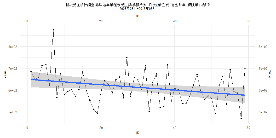
Call:
lm(formula = value ~ ID)

Residuals:
     Min       1Q   Median       3Q      Max
-134.632  -49.679    0.669   35.910  235.273

Coefficients:
            Estimate Std. Error t value            Pr(>|t|)
(Intercept) 649.7988    18.7359  34.682 <0.0000000000000002 ***
ID           -1.2388     0.5431  -2.281              0.0263 *
---
Signif. codes:  0 '***' 0.001 '**' 0.01 '*' 0.05 '.' 0.1 ' ' 1

Residual standard error: 71.04 on 57 degrees of freedom
Multiple R-squared:  0.08364,   Adjusted R-squared:  0.06756
F-statistic: 5.202 on 1 and 57 DF,  p-value: 0.02631


    Two-sample Kolmogorov-Smirnov test

data:  lm_residuals and rnorm(n = length(lm_residuals), mean = 0, sd = sd(lm_residuals))
D = 0.10169, p-value = 0.9239
alternative hypothesis: two-sided


    Durbin-Watson test

data:  value ~ ID
DW = 2.2468, p-value = 0.7939
alternative hypothesis: true autocorrelation is greater than 0


    studentized Breusch-Pagan test

data:  value ~ ID
BP = 0.19822, df = 1, p-value = 0.6562


    Box-Ljung test

data:  lm_residuals
X-squared = 1.4384, df = 1, p-value = 0.2304
Call:
lm(formula = value ~ ID)

Residuals:
    Min      1Q  Median      3Q     Max
-226.13  -83.21   -0.86   69.79  430.37

Coefficients:
            Estimate Std. Error t value            Pr(>|t|)
(Intercept) 691.6489    26.6849  25.919 <0.0000000000000002 ***
ID           -0.2422     0.5869  -0.413               0.681
---
Signif. codes:  0 '***' 0.001 '**' 0.01 '*' 0.05 '.' 0.1 ' ' 1

Residual standard error: 116.7 on 76 degrees of freedom
Multiple R-squared:  0.002236,  Adjusted R-squared:  -0.01089
F-statistic: 0.1703 on 1 and 76 DF,  p-value: 0.681


    Two-sample Kolmogorov-Smirnov test

data:  lm_residuals and rnorm(n = length(lm_residuals), mean = 0, sd = sd(lm_residuals))
D = 0.11538, p-value = 0.6802
alternative hypothesis: two-sided


    Durbin-Watson test

data:  value ~ ID
DW = 2.1483, p-value = 0.7056
alternative hypothesis: true autocorrelation is greater than 0


    studentized Breusch-Pagan test

data:  value ~ ID
BP = 6.5983, df = 1, p-value = 0.01021


    Box-Ljung test

data:  lm_residuals
X-squared = 0.85543, df = 1, p-value = 0.355