Analysis
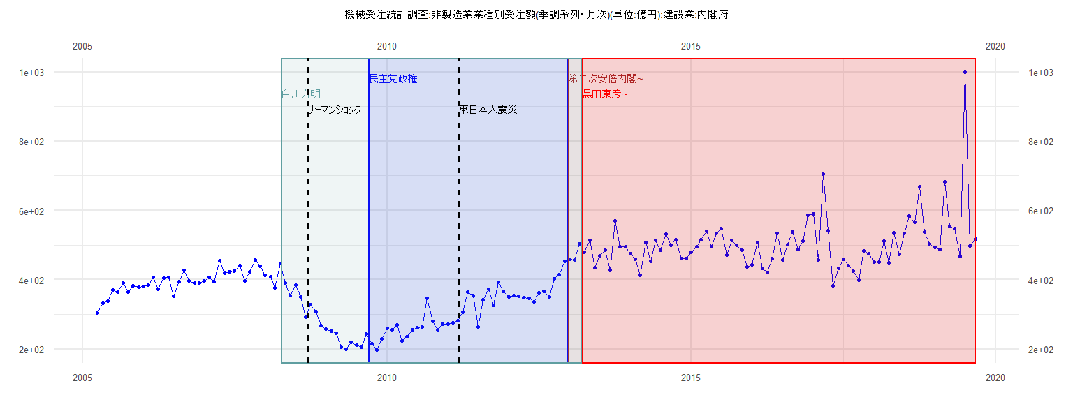
[1] "機械受注統計調査:非製造業業種別受注額(季調系列・月次)(単位:億円):建設業:内閣府"
        Jan    Feb    Mar    Apr    May    Jun    Jul    Aug    Sep    Oct    Nov    Dec
2005                      303.78 331.89 337.70 370.00 365.26 389.88 364.41 381.53 379.02
2006 380.98 383.66 407.11 372.59 404.98 405.85 352.18 394.90 426.39 396.84 389.50 391.07
2007 397.25 406.50 394.05 454.67 418.32 422.49 424.03 441.58 396.86 423.65 456.03 438.80
2008 412.97 408.43 376.10 446.64 390.15 353.57 384.02 349.99 291.68 327.28 307.25 267.55
2009 257.17 251.75 245.22 205.44 199.94 219.56 212.11 204.58 242.88 215.08 197.93 229.45
2010 259.23 255.35 269.52 224.14 234.54 254.97 260.84 263.21 346.47 279.57 255.75 272.53
2011 271.28 275.42 282.26 305.50 363.81 353.47 264.14 342.29 373.03 326.25 392.12 366.12
2012 349.97 353.63 352.81 348.75 345.88 336.31 361.84 366.58 350.00 403.11 414.99 453.46
2013 458.97 456.18 502.71 479.99 512.48 435.56 468.92 484.24 426.28 570.35 494.45 495.94
2014 475.77 459.21 412.04 506.63 453.10 514.31 485.86 531.57 498.48 516.13 460.22 461.15
2015 479.26 494.58 515.09 538.98 496.09 534.25 547.58 471.42 513.65 499.29 484.59 437.61
2016 443.51 507.03 431.95 420.44 461.09 532.88 457.84 501.32 538.57 486.59 512.00 586.07
2017 590.35 456.19 705.76 540.80 381.75 431.87 459.86 440.33 424.70 399.21 482.29 475.01
2018 450.19 451.85 511.57 448.95 535.04 472.72 533.48 584.70 565.50 667.73 538.54 502.84
2019 492.83 487.53 682.67 554.29 548.12 467.65 998.93 497.50 517.41
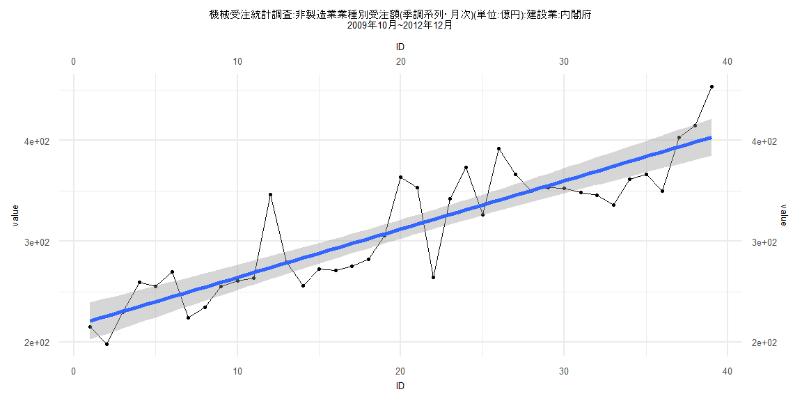
Call:
lm(formula = value ~ ID)

Residuals:
    Min      1Q  Median      3Q     Max
-57.548 -20.108  -4.347  16.171  72.760

Coefficients:
            Estimate Std. Error t value             Pr(>|t|)
(Intercept) 216.1363     9.4210   22.94 < 0.0000000000000002 ***
ID            4.7978     0.4105   11.69   0.0000000000000555 ***
---
Signif. codes:  0 '***' 0.001 '**' 0.01 '*' 0.05 '.' 0.1 ' ' 1

Residual standard error: 28.85 on 37 degrees of freedom
Multiple R-squared:  0.7869,    Adjusted R-squared:  0.7811
F-statistic: 136.6 on 1 and 37 DF,  p-value: 0.00000000000005552


    Two-sample Kolmogorov-Smirnov test

data:  lm_residuals and rnorm(n = length(lm_residuals), mean = 0, sd = sd(lm_residuals))
D = 0.17949, p-value = 0.5622
alternative hypothesis: two-sided


    Durbin-Watson test

data:  value ~ ID
DW = 1.558, p-value = 0.05654
alternative hypothesis: true autocorrelation is greater than 0


    studentized Breusch-Pagan test

data:  value ~ ID
BP = 0.39826, df = 1, p-value = 0.528


    Box-Ljung test

data:  lm_residuals
X-squared = 1.3564, df = 1, p-value = 0.2442
Call:
lm(formula = value ~ ID)

Residuals:
    Min      1Q  Median      3Q     Max
-133.57  -45.33    0.47   26.50  457.12

Coefficients:
            Estimate Std. Error t value             Pr(>|t|)
(Intercept) 461.3158    17.1950  26.828 < 0.0000000000000002 ***
ID            1.0189     0.3643   2.797              0.00648 **
---
Signif. codes:  0 '***' 0.001 '**' 0.01 '*' 0.05 '.' 0.1 ' ' 1

Residual standard error: 76.66 on 79 degrees of freedom
Multiple R-squared:  0.09009,   Adjusted R-squared:  0.07857
F-statistic: 7.822 on 1 and 79 DF,  p-value: 0.00648


    Two-sample Kolmogorov-Smirnov test

data:  lm_residuals and rnorm(n = length(lm_residuals), mean = 0, sd = sd(lm_residuals))
D = 0.23457, p-value = 0.02289
alternative hypothesis: two-sided


    Durbin-Watson test

data:  value ~ ID
DW = 1.9611, p-value = 0.3855
alternative hypothesis: true autocorrelation is greater than 0


    studentized Breusch-Pagan test

data:  value ~ ID
BP = 4.6623, df = 1, p-value = 0.03083


    Box-Ljung test

data:  lm_residuals
X-squared = 0.029393, df = 1, p-value = 0.8639
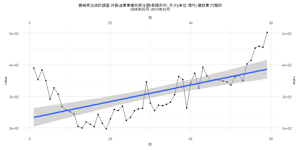
Call:
lm(formula = value ~ ID)

Residuals:
   Min     1Q Median     3Q    Max
-83.33 -43.78 -14.21  34.61 156.18

Coefficients:
            Estimate Std. Error t value             Pr(>|t|)
(Intercept) 231.3383    15.3025  15.118 < 0.0000000000000002 ***
ID            2.6275     0.4436   5.923          0.000000192 ***
---
Signif. codes:  0 '***' 0.001 '**' 0.01 '*' 0.05 '.' 0.1 ' ' 1

Residual standard error: 58.02 on 57 degrees of freedom
Multiple R-squared:  0.381, Adjusted R-squared:  0.3701
F-statistic: 35.08 on 1 and 57 DF,  p-value: 0.0000001922


    Two-sample Kolmogorov-Smirnov test

data:  lm_residuals and rnorm(n = length(lm_residuals), mean = 0, sd = sd(lm_residuals))
D = 0.15254, p-value = 0.5021
alternative hypothesis: two-sided


    Durbin-Watson test

data:  value ~ ID
DW = 0.34397, p-value < 0.00000000000000022
alternative hypothesis: true autocorrelation is greater than 0


    studentized Breusch-Pagan test

data:  value ~ ID
BP = 7.6811, df = 1, p-value = 0.00558


    Box-Ljung test

data:  lm_residuals
X-squared = 32.994, df = 1, p-value = 0.000000009243
Call:
lm(formula = value ~ ID)

Residuals:
    Min      1Q  Median      3Q     Max
-133.50  -46.71    2.09   26.93  456.48

Coefficients:
            Estimate Std. Error t value             Pr(>|t|)
(Intercept) 462.9330    17.8412  25.947 < 0.0000000000000002 ***
ID            1.0463     0.3924   2.666              0.00936 **
---
Signif. codes:  0 '***' 0.001 '**' 0.01 '*' 0.05 '.' 0.1 ' ' 1

Residual standard error: 78.03 on 76 degrees of freedom
Multiple R-squared:  0.08555,   Adjusted R-squared:  0.07352
F-statistic:  7.11 on 1 and 76 DF,  p-value: 0.009362


    Two-sample Kolmogorov-Smirnov test

data:  lm_residuals and rnorm(n = length(lm_residuals), mean = 0, sd = sd(lm_residuals))
D = 0.12821, p-value = 0.546
alternative hypothesis: two-sided


    Durbin-Watson test

data:  value ~ ID
DW = 1.962, p-value = 0.3875
alternative hypothesis: true autocorrelation is greater than 0


    studentized Breusch-Pagan test

data:  value ~ ID
BP = 4.4488, df = 1, p-value = 0.03493


    Box-Ljung test

data:  lm_residuals
X-squared = 0.026032, df = 1, p-value = 0.8718