Analysis
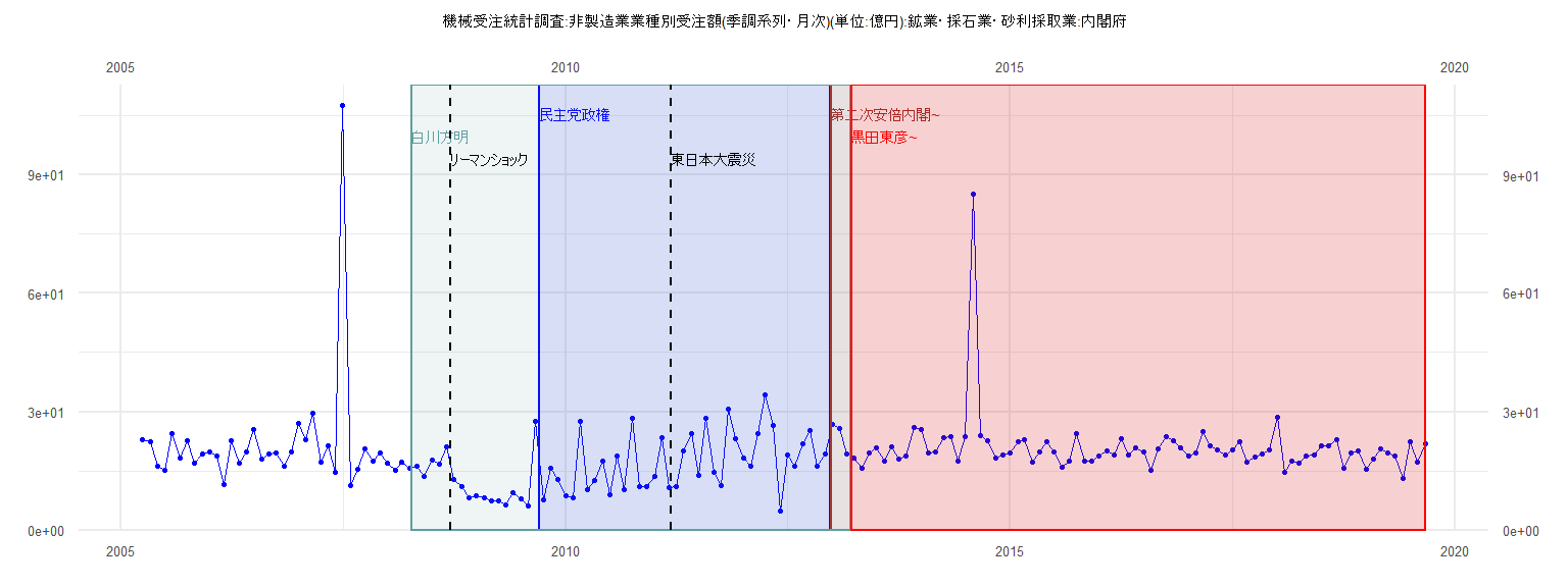
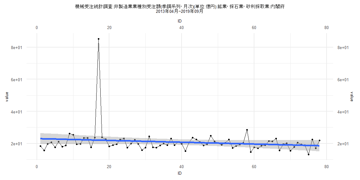
[1] "機械受注統計調査:非製造業業種別受注額(季調系列・月次)(単位:億円):鉱業・採石業・砂利採取業:内閣府"
        Jan    Feb    Mar    Apr    May    Jun    Jul    Aug    Sep    Oct    Nov    Dec
2005                       23.03  22.31  16.32  15.09  24.57  18.20  22.53  16.98  19.26
2006  19.85  18.85  11.65  22.60  16.91  19.94  25.60  17.98  19.24  19.46  16.24  19.76
2007  26.92  23.00  29.72  17.34  21.29  14.77 107.53  11.23  15.44  20.64  17.48  19.63
2008  17.08  15.15  17.15  15.74  16.24  13.73  17.72  16.68  21.04  12.91  11.04   8.20
2009   8.71   8.21   7.40   7.31   6.33   9.57   7.96   6.08  27.61   7.67  15.60  12.97
2010   8.65   8.27  27.64  10.18  12.48  17.38   8.93  18.73  10.39  28.40  11.12  10.95
2011  13.64  23.33  10.87  11.14  20.03  24.54  13.91  28.44  14.77  11.38  30.65  23.23
2012  18.30  16.31  24.54  34.14  26.60   4.96  18.96  16.29  21.92  25.32  16.11  19.42
2013  26.72  25.87  19.26  18.35  15.76  19.68  20.78  17.59  21.23  18.12  18.89  26.12
2014  25.51  19.57  19.78  23.45  23.56  17.60  23.74  85.16  23.86  22.74  18.18  19.00
2015  19.66  22.44  23.02  17.35  19.93  22.35  19.85  15.93  17.53  24.49  17.57  17.53
2016  18.76  20.05  19.06  23.15  18.96  20.93  19.80  15.23  20.59  23.69  22.59  20.96
2017  18.77  19.50  24.90  21.38  20.34  19.15  20.38  22.48  17.17  18.49  19.35  20.31
2018  28.62  14.73  17.61  17.08  18.67  19.09  21.48  21.31  23.00  15.72  19.49  20.07
2019  15.42  17.89  20.52  19.48  18.90  13.17  22.42  17.14  21.93
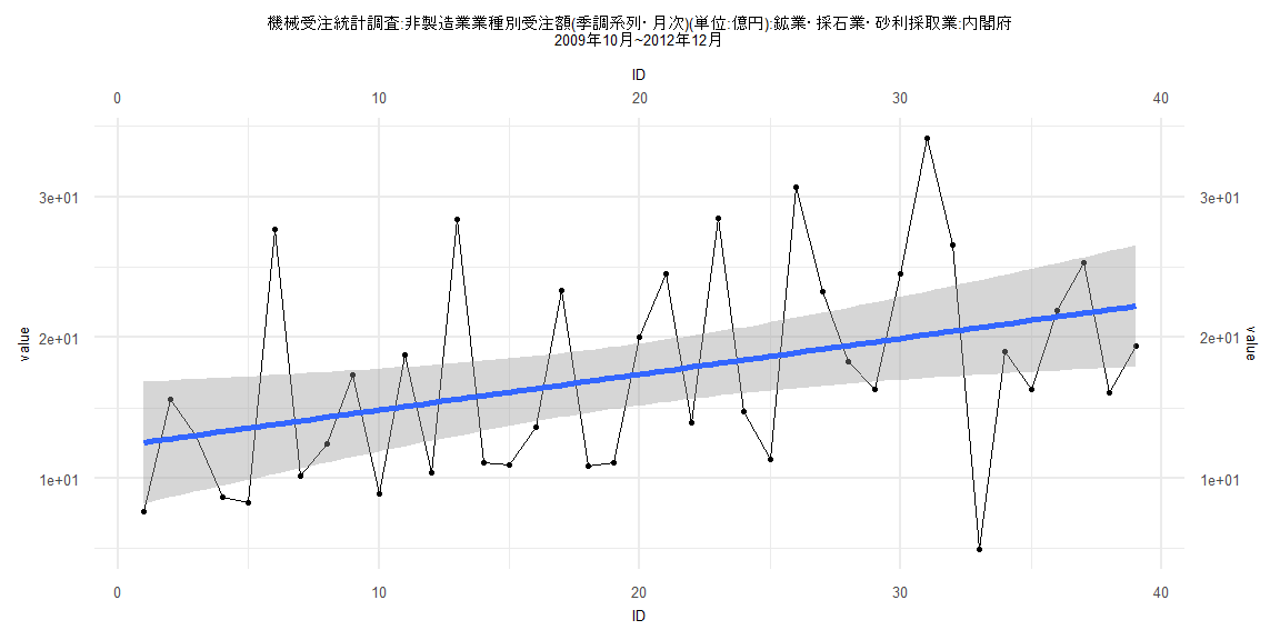
Call:
lm(formula = value ~ ID)

Residuals:
    Min      1Q  Median      3Q     Max
-15.743  -4.899  -1.998   3.846  13.947

Coefficients:
            Estimate Std. Error t value   Pr(>|t|)
(Intercept) 12.28957    2.21531   5.548 0.00000257 ***
ID           0.25496    0.09653   2.641      0.012 *
---
Signif. codes:  0 '***' 0.001 '**' 0.01 '*' 0.05 '.' 0.1 ' ' 1

Residual standard error: 6.785 on 37 degrees of freedom
Multiple R-squared:  0.1586,    Adjusted R-squared:  0.1359
F-statistic: 6.976 on 1 and 37 DF,  p-value: 0.01203


    Two-sample Kolmogorov-Smirnov test

data:  lm_residuals and rnorm(n = length(lm_residuals), mean = 0, sd = sd(lm_residuals))
D = 0.20513, p-value = 0.3888
alternative hypothesis: two-sided


    Durbin-Watson test

data:  value ~ ID
DW = 2.3571, p-value = 0.8319
alternative hypothesis: true autocorrelation is greater than 0


    studentized Breusch-Pagan test

data:  value ~ ID
BP = 0.35636, df = 1, p-value = 0.5505


    Box-Ljung test

data:  lm_residuals
X-squared = 1.4849, df = 1, p-value = 0.223
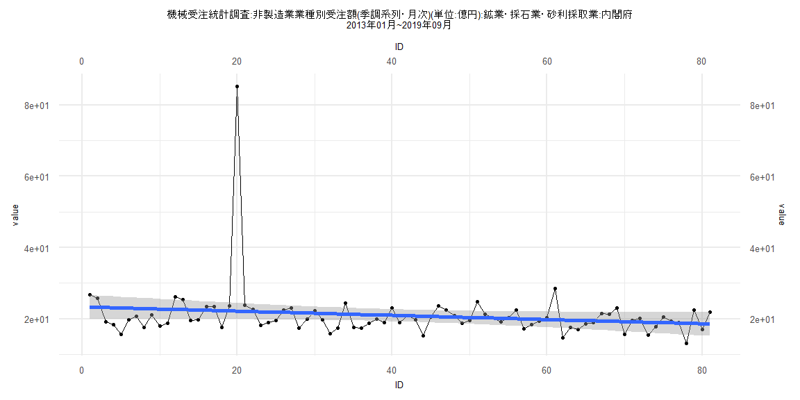
Call:
lm(formula = value ~ ID)

Residuals:
   Min     1Q Median     3Q    Max
-7.326 -2.965 -0.931  1.232 62.959

Coefficients:
            Estimate Std. Error t value            Pr(>|t|)
(Intercept) 23.38134    1.72973   13.52 <0.0000000000000002 ***
ID          -0.05901    0.03665   -1.61               0.111
---
Signif. codes:  0 '***' 0.001 '**' 0.01 '*' 0.05 '.' 0.1 ' ' 1

Residual standard error: 7.712 on 79 degrees of freedom
Multiple R-squared:  0.03178,   Adjusted R-squared:  0.01952
F-statistic: 2.593 on 1 and 79 DF,  p-value: 0.1113


    Two-sample Kolmogorov-Smirnov test

data:  lm_residuals and rnorm(n = length(lm_residuals), mean = 0, sd = sd(lm_residuals))
D = 0.33333, p-value = 0.0002198
alternative hypothesis: two-sided


    Durbin-Watson test

data:  value ~ ID
DW = 1.8627, p-value = 0.2308
alternative hypothesis: true autocorrelation is greater than 0


    studentized Breusch-Pagan test

data:  value ~ ID
BP = 0.88401, df = 1, p-value = 0.3471


    Box-Ljung test

data:  lm_residuals
X-squared = 0.36898, df = 1, p-value = 0.5436
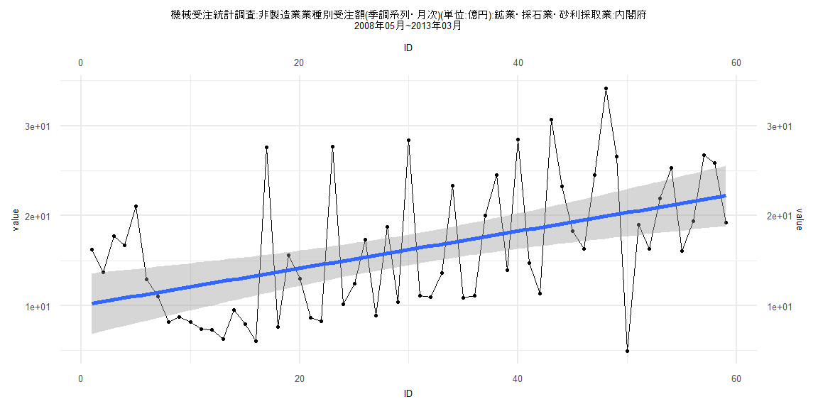
Call:
lm(formula = value ~ ID)

Residuals:
    Min      1Q  Median      3Q     Max
-15.382  -5.177  -2.160   4.485  14.210

Coefficients:
            Estimate Std. Error t value    Pr(>|t|)
(Intercept) 10.02709    1.71715   5.839 0.000000263 ***
ID           0.20630    0.04978   4.144    0.000114 ***
---
Signif. codes:  0 '***' 0.001 '**' 0.01 '*' 0.05 '.' 0.1 ' ' 1

Residual standard error: 6.511 on 57 degrees of freedom
Multiple R-squared:  0.2316,    Adjusted R-squared:  0.2181
F-statistic: 17.18 on 1 and 57 DF,  p-value: 0.0001143


    Two-sample Kolmogorov-Smirnov test

data:  lm_residuals and rnorm(n = length(lm_residuals), mean = 0, sd = sd(lm_residuals))
D = 0.30508, p-value = 0.00792
alternative hypothesis: two-sided


    Durbin-Watson test

data:  value ~ ID
DW = 2.1174, p-value = 0.6245
alternative hypothesis: true autocorrelation is greater than 0


    studentized Breusch-Pagan test

data:  value ~ ID
BP = 0.17374, df = 1, p-value = 0.6768


    Box-Ljung test

data:  lm_residuals
X-squared = 0.28673, df = 1, p-value = 0.5923
Call:
lm(formula = value ~ ID)

Residuals:
   Min     1Q Median     3Q    Max
-7.214 -2.884 -0.970  1.225 63.037

Coefficients:
            Estimate Std. Error t value            Pr(>|t|)
(Intercept) 23.08720    1.79123   12.89 <0.0000000000000002 ***
ID          -0.05672    0.03940   -1.44               0.154
---
Signif. codes:  0 '***' 0.001 '**' 0.01 '*' 0.05 '.' 0.1 ' ' 1

Residual standard error: 7.834 on 76 degrees of freedom
Multiple R-squared:  0.02655,   Adjusted R-squared:  0.01374
F-statistic: 2.073 on 1 and 76 DF,  p-value: 0.1541


    Two-sample Kolmogorov-Smirnov test

data:  lm_residuals and rnorm(n = length(lm_residuals), mean = 0, sd = sd(lm_residuals))
D = 0.24359, p-value = 0.01923
alternative hypothesis: two-sided


    Durbin-Watson test

data:  value ~ ID
DW = 1.8668, p-value = 0.2392
alternative hypothesis: true autocorrelation is greater than 0


    studentized Breusch-Pagan test

data:  value ~ ID
BP = 1.0764, df = 1, p-value = 0.2995


    Box-Ljung test

data:  lm_residuals
X-squared = 0.32273, df = 1, p-value = 0.57